We can easily visualize multiple dimensions of our data with seaborn and matplotlib. Let’s look at the penguin dataset to demonstrate how to visualize multiple dimensions.
import pandas as pdurl ="https://raw.githubusercontent.com/dataprofessor/data/refs/heads/master/penguins_cleaned.csv"df = pd.read_csv(url)df.head()
species
island
bill_length_mm
bill_depth_mm
flipper_length_mm
body_mass_g
sex
0
Adelie
Torgersen
39.1
18.7
181
3750
male
1
Adelie
Torgersen
39.5
17.4
186
3800
female
2
Adelie
Torgersen
40.3
18.0
195
3250
female
3
Adelie
Torgersen
36.7
19.3
193
3450
female
4
Adelie
Torgersen
39.3
20.6
190
3650
male
Let’s begin by visualizing the mean base salary across different positions. To do this, we will use the catplot() function from seaborn. The catplot() function allows us to create categorical plots with multiple dimensions by using the hue parameter. It also allows us to create a variety of different plot types by setting the kind parameter.
The catplot() function gives us 8 options to choose from for the kind parameter: strip (the default parameter), swarm, box, violin, boxen, point, bar, and count. For this example, we will use the bar kind to create a bar chart that compares the mean base salary across different positions, with an additional dimension for guaranteed compensation represented by color.
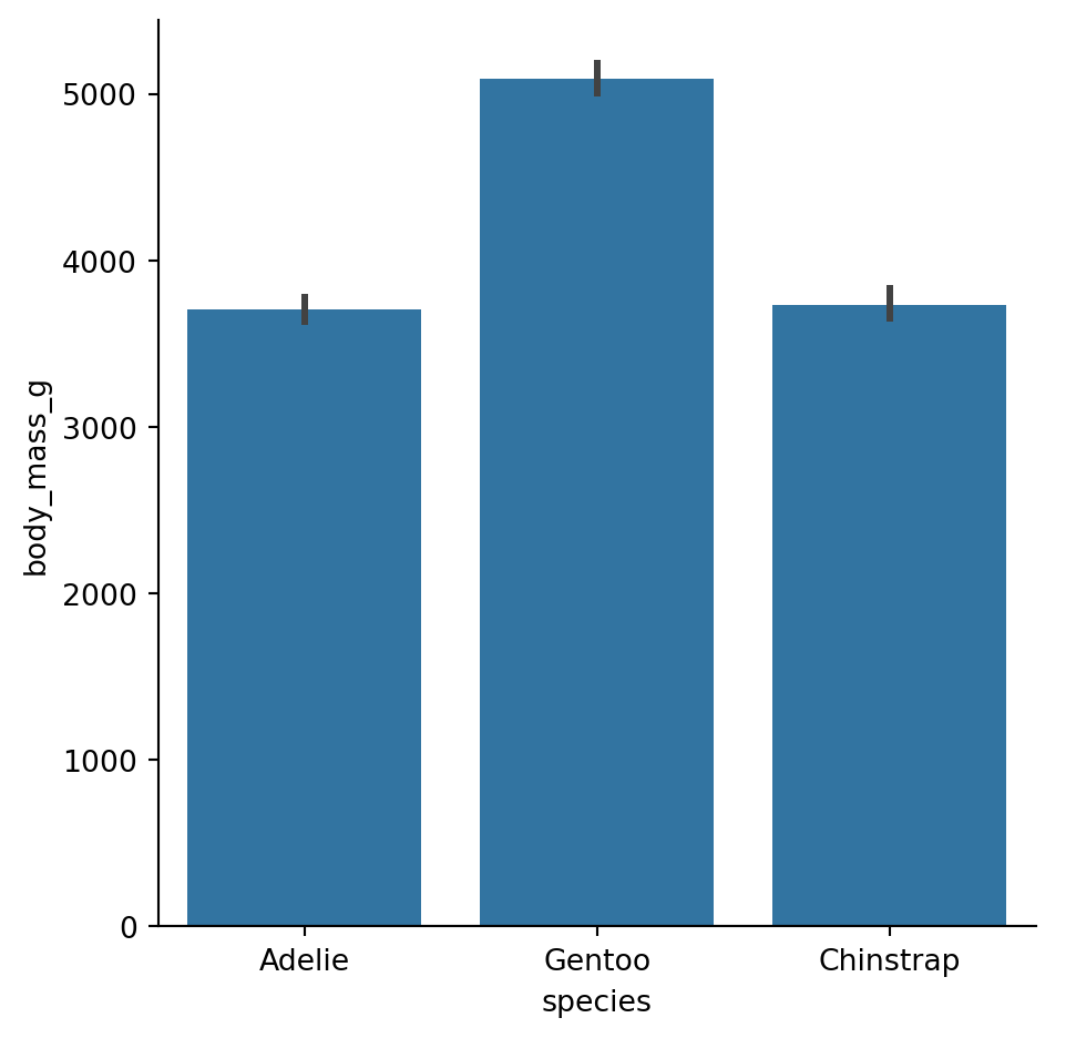
import seaborn as snsimport matplotlib.pyplot as pltplt.figure(figsize=(8, 6))sns.catplot(data=df, x="species", y="body_mass_g", kind="bar")
<Figure size 768x576 with 0 Axes>
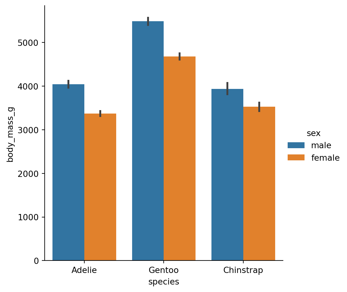
We can see we created a simple bar chart that compares the mean body mass across different species of penguins. The catplot() function automatically calculates the mean for us and creates the bar chart. It also makes it easy to add additional dimensions to our visualization. By using the hue parameter, we can add another categorical variable to our plot. Let’s add the sex variable as a hue to our bar chart.
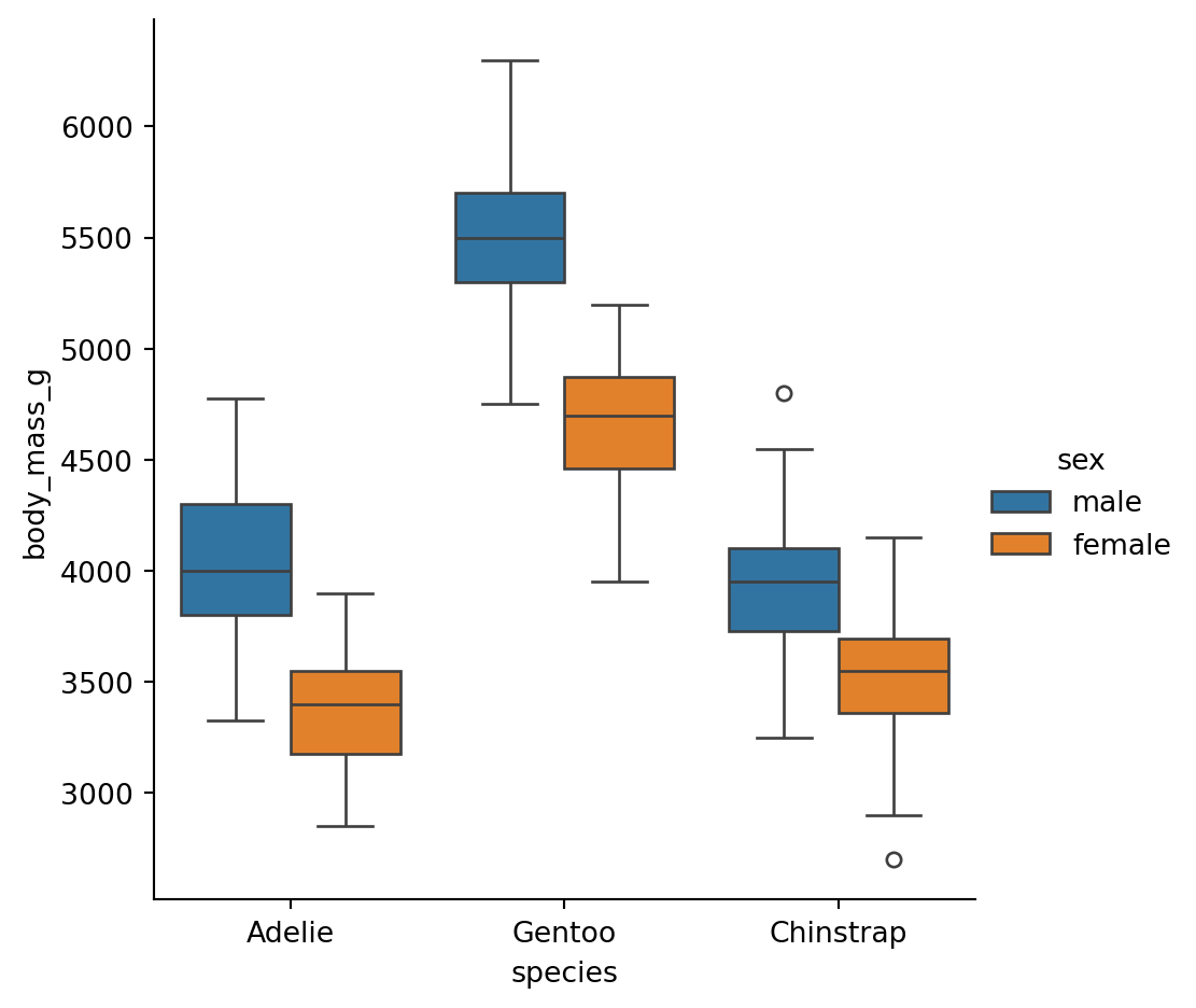
But there is more, we can start changing how we visualize our data by changing the kind parameter. Let’s change the kind parameter to box to create a box plot that compares the body mass across different species of penguins, with an additional dimension for sex represented by color.
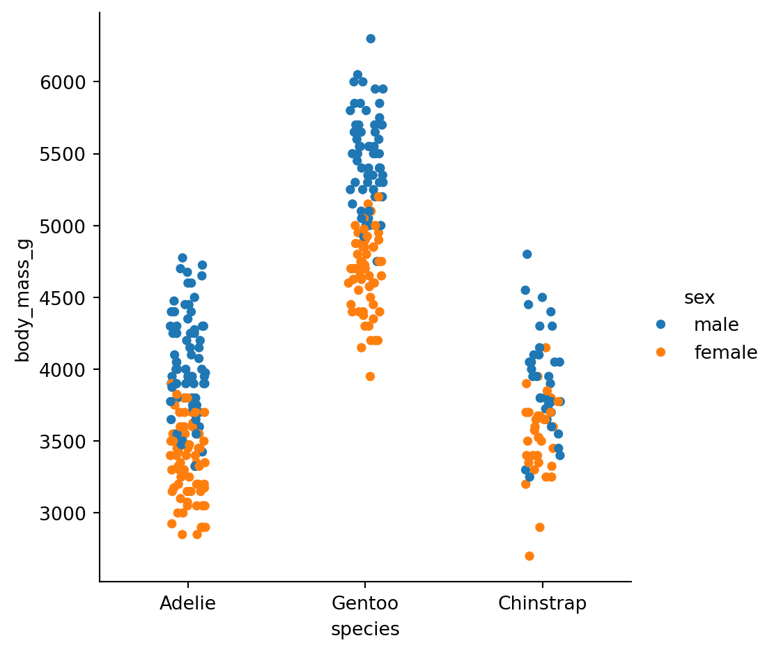
If we want to visualize the actual data points instead of summary statistics, we can use the strip or swarm kinds. The strip kind creates a scatter plot where the points are jittered to avoid overlap, while the swarm kind creates a scatter plot where the points are adjusted to avoid overlap. Let’s create a strip plot that compares the body mass across different species of penguins, with an additional dimension for sex represented by color.
Let’s now look at each of the others kinds available in the catplot() function.
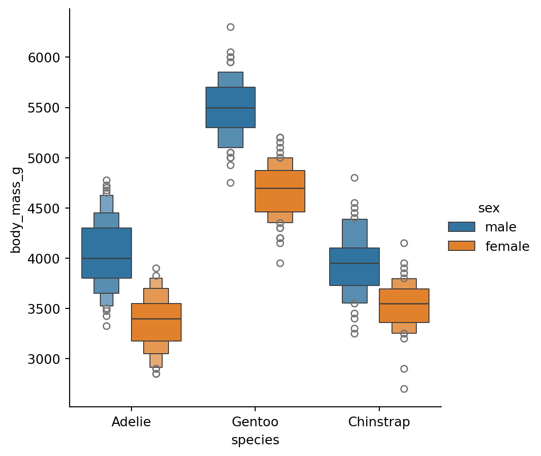
Boxen Plot
The boxen kind creates a boxen plot, which is similar to a box plot but provides more information about the distribution of the data. Let’s create a boxen plot that compares the body mass across different species of penguins, with an additional dimension for sex represented by color.
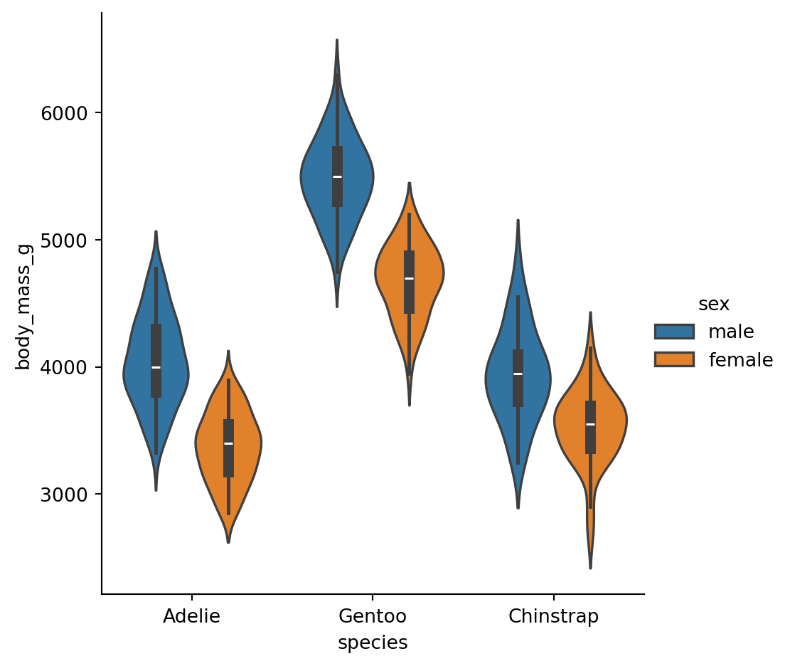
The violin kind creates a violin plot, which is similar to a box plot but also shows the kernel density estimation of the data. Let’s create a violin plot that compares the body mass across different species of penguins, with an additional dimension for sex represented by color.
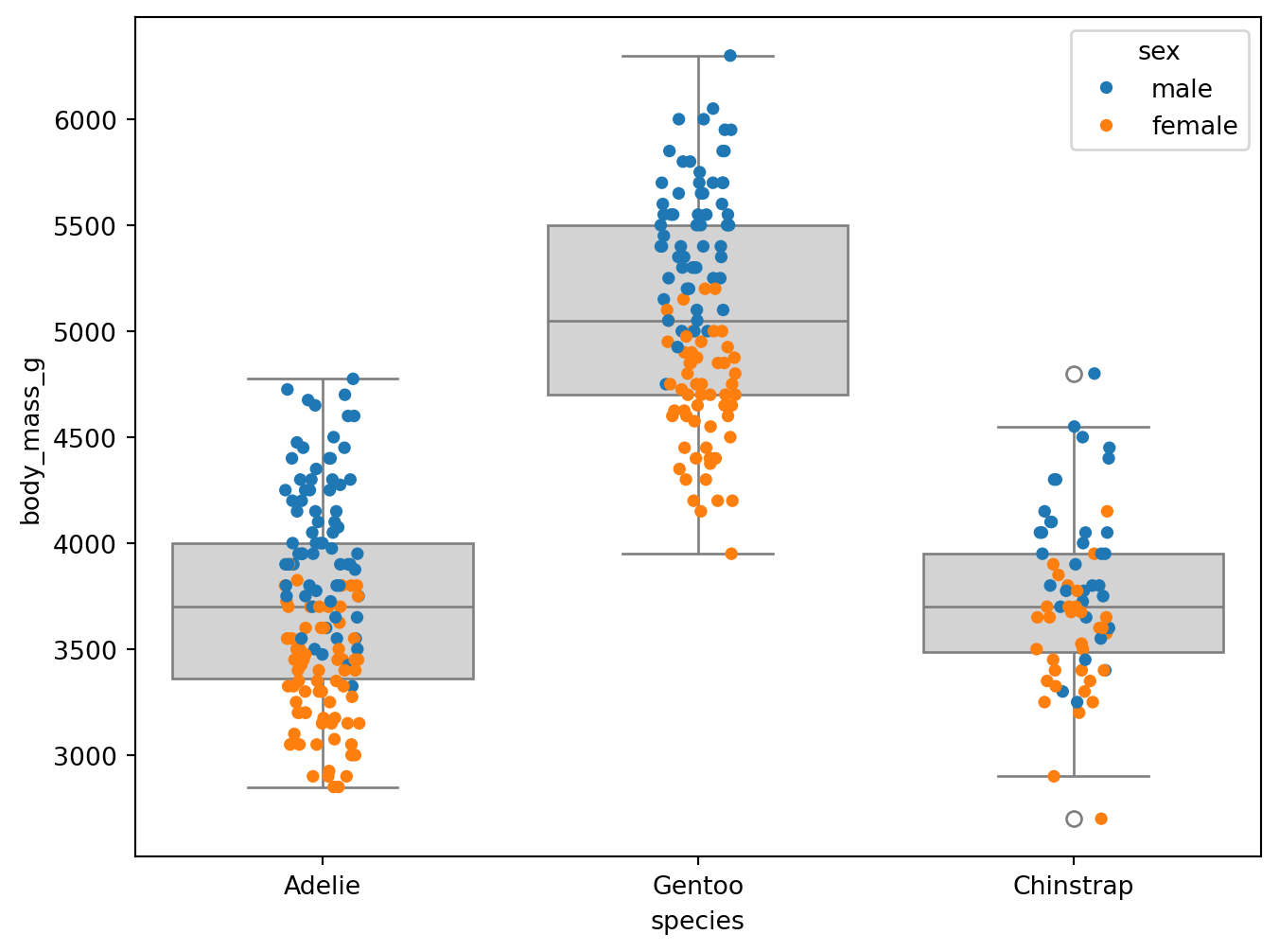
We can also build plots on top of each other as well. But to do so, we also need to use the specific named plots as opposed to catplot() because catplot() is a figure level function (it creates a new figure each time). But we can overlay a strip plot on top of a box plot using stripplot() and boxplot() to represent the locations of each data and represent the interquartile range. Let’s create a box plot that compares the body mass across different species of penguins, with an additional dimension for sex represented by color.
To do this, we will first create the box plot with no hue, and set the color to lightgray. Then, we will create the strip plot on top of the box plot, setting the hue to sex to represent the different sexes.
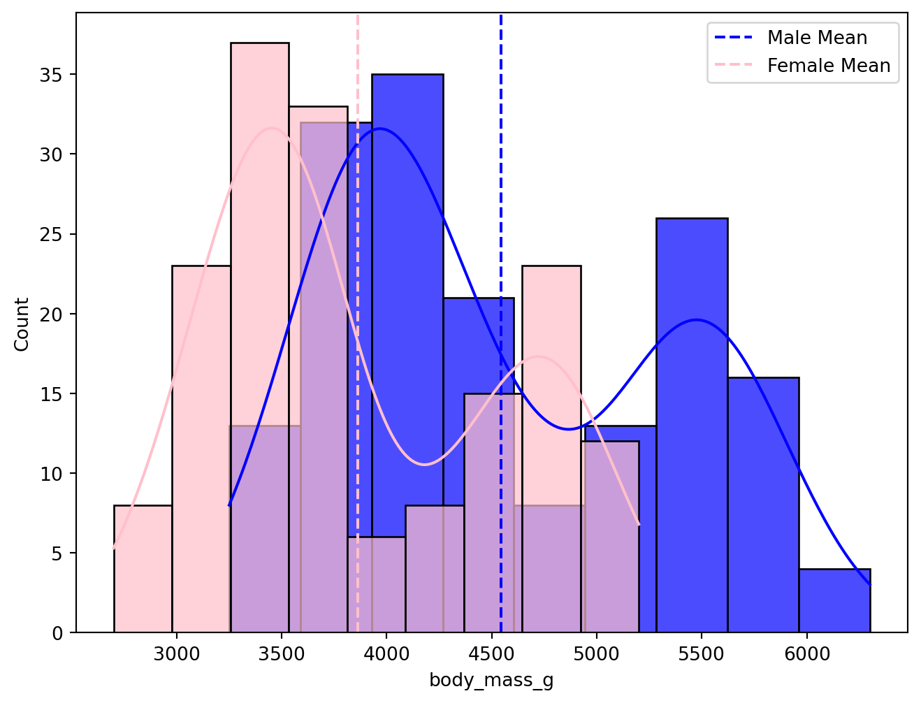
We can similarly overlay two histograms as well. Let’s create a histogram that compares the body mass across different species of penguins, with an additional dimension for sex represented by color.