11.2 Multiple Dimension Visualizations

Bivariate N2N Visualizations

Sometimes we want to visualize relationships across multiple dimensions (think categories or groups) in our bivariate N2N plots. This can be achieved by creating separate plots for each dimension or by using facets to display multiple dimensions within a single plot.

For instance, let’s look at our penguin dataset again.

import pandas as pd
import matplotlib.pyplot as plt
import seaborn as sns

# Load the penguin dataset
url = "https://raw.githubusercontent.com/dataprofessor/data/refs/heads/master/penguins_cleaned.csv"
penguins = pd.read_csv(url)

penguins.head()

	species	island	bill_length_mm	bill_depth_mm	flipper_length_mm	body_mass_g	sex
0	Adelie	Torgersen	39.1	18.7	181	3750	male
1	Adelie	Torgersen	39.5	17.4	186	3800	female
2	Adelie	Torgersen	40.3	18.0	195	3250	female
3	Adelie	Torgersen	36.7	19.3	193	3450	female
4	Adelie	Torgersen	39.3	20.6	190	3650	male

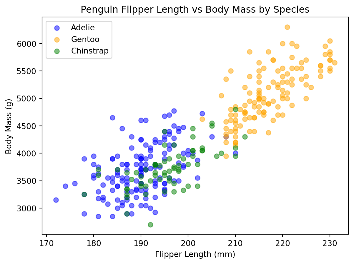
We can see that the dataset contains a categorical variable species that indicates the species of each penguin. We can create separate scatter plots for each species to visualize the relationship between flipper length and body mass.

penguins['species'].unique()

array(['Adelie', 'Gentoo', 'Chinstrap'], dtype=object)

When we look at the categories available in species, we can create separate scatter plots for each species and place them all on the same figure. This would be considered a three dimensional visualization (flipper length, body mass, and species).

plt.figure(figsize=(7, 5))
colors = ['blue', 'orange', 'green']
for species in penguins['species'].unique():
    subset = penguins[penguins['species'] == species]
    plt.scatter(
        subset['flipper_length_mm'], 
        subset['body_mass_g'], 
        alpha=0.5, 
        label=species, 
        color=colors.pop(0) # remember pop returns and removes the first item from the list
        )  
plt.xlabel('Flipper Length (mm)')
plt.ylabel('Body Mass (g)')
plt.title('Penguin Flipper Length vs Body Mass by Species')
plt.legend()
plt.show()

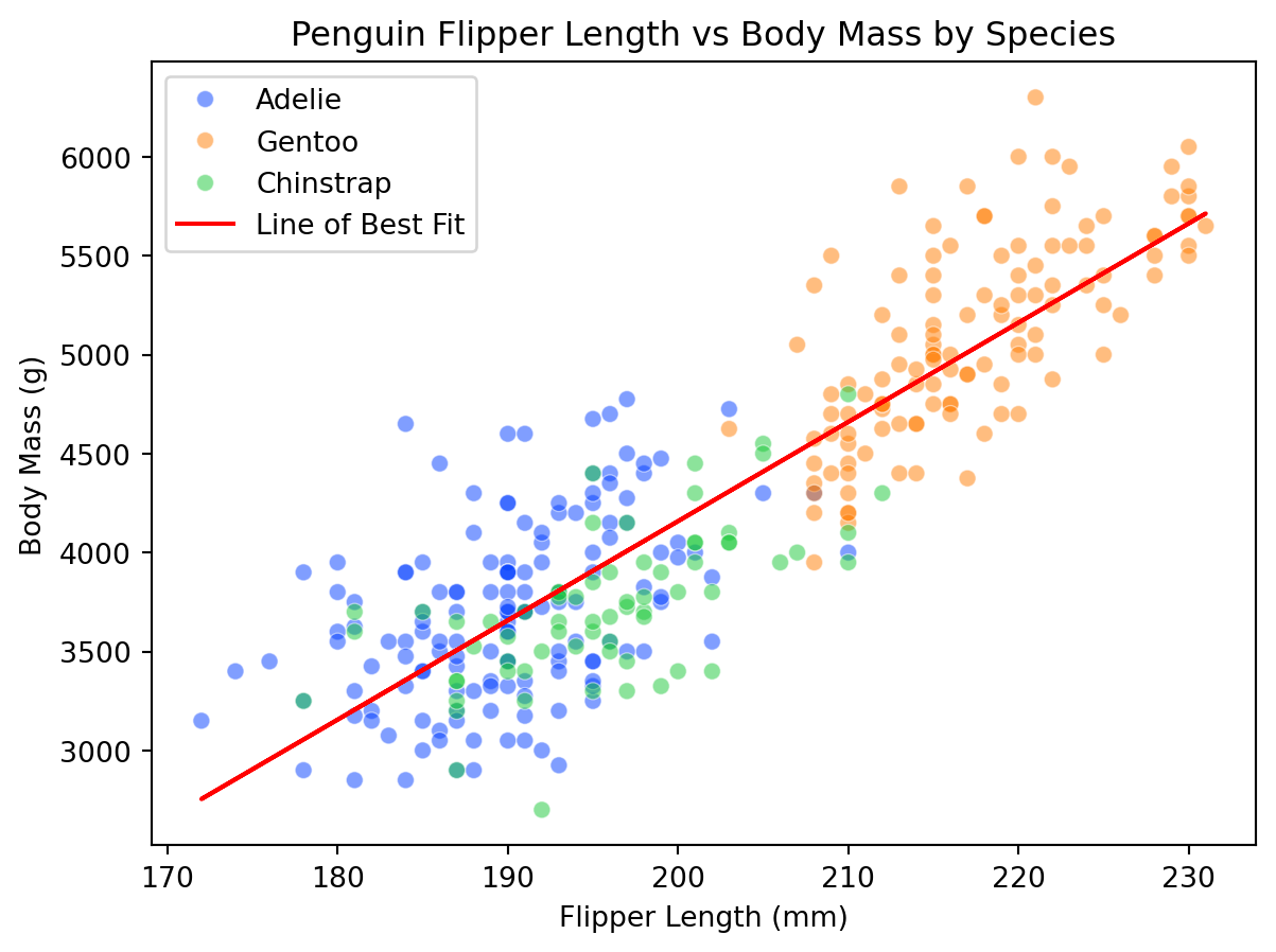
We can also do this using seaborn's scatterplot function, which allows us to easily map the hue parameter to the species variable. Unfortunately, however, seaborn does not have a built-in way to add a line of best fit that accounts for multiple categories in a single plot. We can, however, calculate the line of best fit for the entire dataset and overlay it on the scatter plot.

from scipy import stats

plt.figure(figsize=(7, 5))
scat = sns.scatterplot(
    data=penguins,
    x="flipper_length_mm",
    y="body_mass_g",
    hue="species",
    alpha=0.5,
    palette="bright",  # premade palette
    # palette=["blue", "orange", "green"], # can also include our own palette
)
m, b, r, p, err = stats.linregress(
    penguins["flipper_length_mm"], penguins["body_mass_g"]
)
line = m * penguins["flipper_length_mm"] + b
plt.plot(penguins["flipper_length_mm"], line, color="red", label="Line of Best Fit")
scat.set(xlabel="Flipper Length (mm)", ylabel="Body Mass (g)")
plt.title("Penguin Flipper Length vs Body Mass by Species")
plt.legend()
plt.show()

We can see from this plot that while there is a general trend of increasing body mass with flipper length, the relationship varies by species. Each species has its own cluster of points, and the overall line of best fit may not accurately represent the relationship for each individual species.

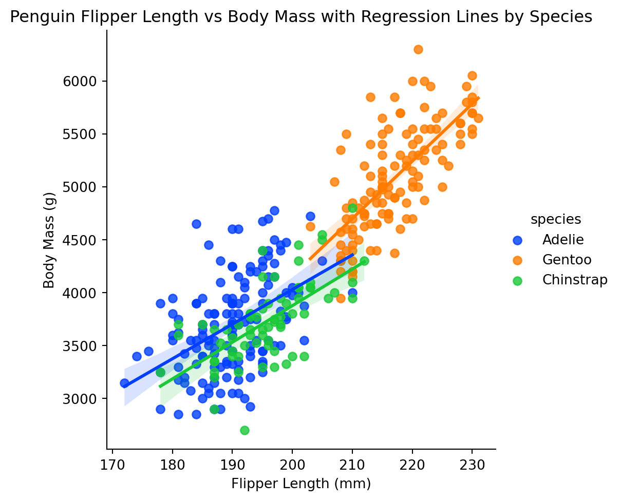
To make this a bit clearer, we can use seaborn's lmplot function, which allows us to create separate regression lines for each species using the hue parameter.

Here is the explanation of the difference between regplot and lmplot from the seaborn documentation:

These functions draw similar plots, but regplot() is an axes-level function, and lmplot() is a figure-level function. Additionally, regplot() accepts the x and y variables in a variety of formats including simple numpy arrays, pandas.Series objects, or as references to variables in a pandas.DataFrame object passed to data. In contrast, lmplot() has data as a required parameter and the x and y variables must be specified as strings. Finally, only lmplot() has hue as a parameter.

plt.figure(figsize=(7, 5))
lm = sns.lmplot(
    data=penguins,
    x="flipper_length_mm",
    y="body_mass_g",
    hue="species",
    palette="bright",
)
lm.set(xlabel="Flipper Length (mm)", ylabel="Body Mass (g)")
plt.title("Penguin Flipper Length vs Body Mass with Regression Lines by Species")
plt.show()

<Figure size 672x480 with 0 Axes>

Four Dimension Visualizations

Now we can also include a fourth dimension by varying the

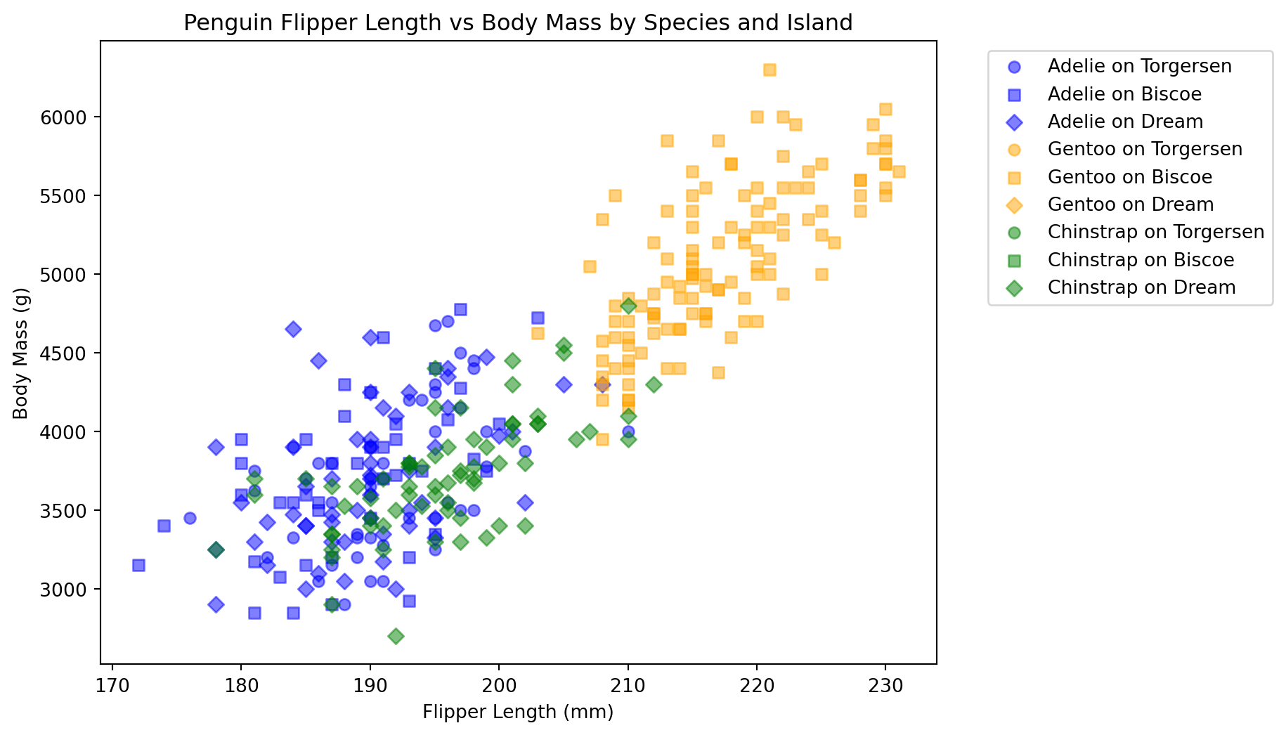
We will use different markers for each island in addition to different colors for each species.

species = penguins["species"].unique()
islands = penguins["island"].unique()
colors = ["blue", "orange", "green"]
markers = ["o", "s", "D"]
plt.figure(figsize=(8, 6))
for spec in species:
    for island in islands:
        subset = penguins[
            (penguins["species"] == spec) & (penguins["island"] == island)
        ]
        plt.scatter(
            subset["flipper_length_mm"],
            subset["body_mass_g"],
            alpha=0.5,
            label=f"{spec} on {island}",
            color=colors[
                list(species).index(spec)
            ],  # returns index of species to select color
            marker=markers[
                list(islands).index(island)
            ],  # returns index of island to select marker
        )
plt.xlabel("Flipper Length (mm)")
plt.ylabel("Body Mass (g)")
plt.title("Penguin Flipper Length vs Body Mass by Species and Island")
plt.legend(bbox_to_anchor=(1.05, 1), loc="upper left")
plt.show()

Once again, we can see that the relationship between flipper length and body mass varies not only by species but also by island. Each combination of species and island has its own cluster of points, highlighting the complexity of the relationships in the dataset.