9.1 Anatomy of a Visualization

Visualizing Univariate Data

Before we get into specific ways to visualize univariate data, let’s take a moment to get acquainted with Matplotlib and the anatomy of a visualization. Matplotlib is a widely used plotting library in Python that provides a flexible way to create static, animated, and interactive visualizations. Understanding the basic components of a Matplotlib plot will help you customize and enhance your visualizations effectively.

Moreover, it has become the principal building block on which other visualization libraries are built. For instance, Seaborn is a statistical data visualization library that is built on top of Matplotlib and provides a high-level interface for drawing attractive and informative statistical graphics. We will work with both Matplotlib and Seaborn in this and the following chapters, but it is good to understand the basics of Matplotlib first. Any further customization of visualizations will need to be done with Matplotlib commands.

To begin, we will import matplotlib.pyplot as plt, which is the conventional alias used by the community. If you have not already installed Matplotlib, you can do so with Anaconda Navigator or by running uv matplotlib in your terminal.

To begin, we will be working with this dataset, which contains sales data for a fictional coffee shop. Please, download the CSV from the provided link and place it in the same directory that you will be running this code. Now let’s open the data and look at it quickly, so we can decide what we want to visualize.

import pandas as pd
import matplotlib.pyplot as plt

# Load the dataset
coffee_sales = pd.read_csv("coffee_sales.csv")
coffee_sales.head()

	hour_of_day	cash_type	money	coffee_name	Time_of_Day	Weekday	Month_name	Weekdaysort	Monthsort	Date	Time
0	10	card	38.7	Latte	Morning	Fri	Mar	5	3	2024-03-01	10:15:50.520000
1	12	card	38.7	Hot Chocolate	Afternoon	Fri	Mar	5	3	2024-03-01	12:19:22.539000
2	12	card	38.7	Hot Chocolate	Afternoon	Fri	Mar	5	3	2024-03-01	12:20:18.089000
3	13	card	28.9	Americano	Afternoon	Fri	Mar	5	3	2024-03-01	13:46:33.006000
4	13	card	38.7	Latte	Afternoon	Fri	Mar	5	3	2024-03-01	13:48:14.626000

Basics of Visualizations in Matplotlib

Maptplotlib uses a state-based interface, meaning that it keeps track of the current figure and axes, and each plotting command modifies the current figure. Due to this design, we do not need to create a variable to hold the figure or axes unless we want to customize them further. The only exception to this is when we build multiple plots at once, which we will see later.

Figure: The entire window or page that contains the plot(s). You can think of it as a canvas where all the elements of the plot are drawn. You can create a figure using plt.figure().
1. Arguments:
  - figsize: A tuple specifying the width and height of the figure in inches. For example, figsize=(10, 6) creates a figure that is 10 inches wide and 6 inches tall.
Axes: The area where the data is plotted. A figure can contain multiple axes (subplots). Each axes has its own coordinate system and can contain multiple plots. You can create axes using plt.subplot() or plt.subplots().
1. Arguments:
  - figsize: A tuple specifying the width and height of the figure in inches. For example, figsize=(10, 6) creates a figure that is 10 inches wide and 6 inches tall.
  - nrows: Number of rows of subplots in the figure.
  - ncols: Number of columns of subplots in the figure.
  - index: The index of the subplot to create (starting from 1).
Plot Elements: These include the actual data representations, such as lines, bars, points, etc. You can create these elements using various plotting functions like plt.plot(), plt.bar(), plt.scatter(), etc.
Labels and Titles: These provide context to the plot, including the title of the plot, labels for the x-axis and y-axis, and legends to differentiate between multiple data series. You can add these using plt.title(), plt.xlabel(), plt.ylabel(), and plt.legend().
Ticks and Grid: Ticks are the markers along the axes that indicate the scale of the plot. Grids are optional lines that can be added to the plot to improve readability. You can customize ticks using plt.xticks() and plt.yticks(), and add a grid using plt.grid().

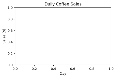
We will learn more about these components as we move forward. For now, we need to understand how to construct the basic structures of a visualization. We need a figure, labels, a title, and ticks. Let’s create a simple line plot to illustrate these components.

plt.figure(figsize=(5, 3))  # Creates the canvas
plt.xlabel("Day")  # Adds x-axis label to the current figure
plt.ylabel("Sales ($)")  # Adds y-axis label to the current figure
plt.title("Daily Coffee Sales")  # Adds a title to the current figure
plt.show()  # Displays the current figure

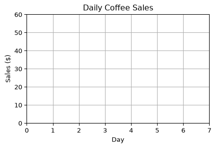
So far, this is a fairly ugly plot. We can change the x-limit and the y-limit to make it look a bit better—so that we can set the total width and height by the max and min range. We can do this using the plt.xlim() and plt.ylim() functions, which allow us to set the limits of the x-axis and y-axis, respectively. Both plt.xlim() and plt.ylim() take two arguments: the lower limit and the upper limit. In addition, we can add grid lines to the plot using the plt.grid() function, which improves readability by adding horizontal and vertical lines across the plot.

plt.figure(figsize=(5, 3))  # Creates the canvas
plt.xlabel("Day")  # Adds x-axis label to the current figure
plt.ylabel("Sales ($)")  # Adds y-axis label to the current figure
plt.title("Daily Coffee Sales")  # Adds a title to the current figure
plt.xlim(0, 7)  # Sets the x-axis limits
plt.ylim(0, 60)  # Sets the y-axis limits
plt.grid(True)  # Adds grid lines to the current figure
plt.show()  # Displays the current figure

Notice that Matplotlib maintains a “current” figure that gets modified by each command. We created the figure with plt.figure(), then added labels and a title, set the limits, and added grid lines. Each command modifies the current figure, and finally, we display the figure with plt.show(). Moreover, it also manages the locations of the ticks automatically, so we don’t need to set them manually unless we want to customize them further.

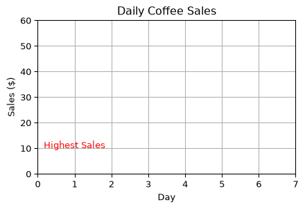
We have the basics of a visualization. We have a figure with a title and axis labels, but we don’t have any data plotted yet. Now let’s add some text to our plot to indicate some information about the data as well. To do this we can use the plt.text() function, which allows us to place text at an arbitrary position on the Axes. The function takes the x and y coordinates of the text position, the text string, and optional parameters for font size, color, and alignment.

plt.figure(figsize=(5, 3))  # Creates the canvas
plt.xlabel("Day")  # Adds x-axis label to the current figure
plt.ylabel("Sales ($)")  # Adds y-axis label to the current figure
plt.title("Daily Coffee Sales")  # Adds a title to the current figure
plt.xlim(0, 7)  # Sets the x-axis limits
plt.ylim(0, 60)  # Sets the y-axis limits
plt.grid(True)  # Adds grid lines to the current figure
text_x = 1  # x-coordinate for the text
text_y = 10  # y-coordinate for the text
text_str = "Highest Sales"  # Text to display
plt.text(
    text_x, text_y, text_str, fontsize=10, color="red", ha="center"
)  # Adds text to the current figure
plt.show()  # Displays the current figure

This is a simple example of how to add text to a plot. The coordinates (1,10) are in data coordinates, meaning they correspond to the data values on the axes. You can adjust these values to position the text where you want it on the plot. In addition, notice that the text is centered horizontally at the specified x-coordinate because we set ha="center". You can change this to "left" or "right" to align the text differently.

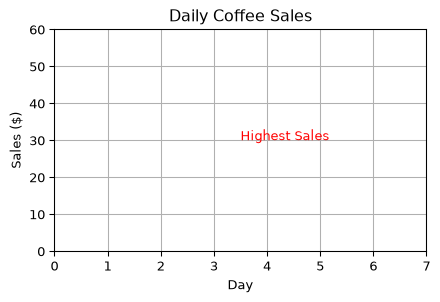
We can also change the location of the text by using the transform argument. This argument allows us to specify the coordinate system for the text position. For example, we can use plt.gca().transAxes to specify that the coordinates are in axes coordinates, where (0, 0) is the bottom-left corner of the axes and (1, 1) is the top-right corner. It effectively allows us to position the text relative to the axes, regardless of the data limits as percentages.

plt.figure(figsize=(5, 3))  # Creates the canvas
plt.xlabel("Day")  # Adds x-axis label to the current figure
plt.ylabel("Sales ($)")  # Adds y-axis label to the current figure
plt.title("Daily Coffee Sales")  # Adds a title to the current figure
plt.xlim(0, 7)  # Sets the x-axis limits
plt.ylim(0, 60)  # Sets the y-axis limits
plt.grid(True)  # Adds grid lines to the current figure
text_x = 0.5  # x-coordinate for the text
text_y = 0.5  # y-coordinate for the text
text_str = "Highest Sales"  # Text to display
plt.text(
    text_x,
    text_y,
    text_str,
    fontsize=10,
    color="red",
    transform=plt.gca().transAxes,  # use axis coordinates
    ha="left",  # changed alignment to left
)  # Adds text to the current figure
plt.show()  # Displays the current figure