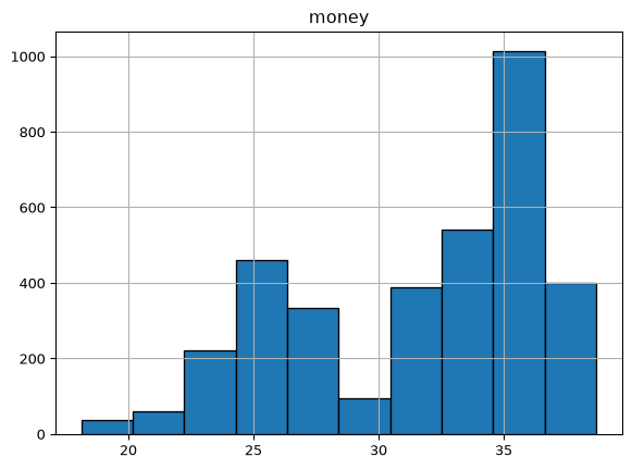
One of the easiest ways to represent the distribution of a single variable is to use a histogram. A histogram is a type of bar chart that represents the frequency distribution of a continuous variable by dividing the data into intervals, or “bins,” and counting how many data points fall into each bin.
Histograms in Pandas
To begin exploring the ways we can create histograms, we will keep using the coffee sales dataset from the previous section. If you have not already downloaded the dataset, please do so from this link and place it in the same directory that you will be running this code. Now let’s load the data and take a quick look at it.
import pandas as pddf = pd.read_csv("coffee_sales.csv")df.head()
hour_of_day
cash_type
money
coffee_name
Time_of_Day
Weekday
Month_name
Weekdaysort
Monthsort
Date
Time
0
10
card
38.7
Latte
Morning
Fri
Mar
5
3
2024-03-01
10:15:50.520000
1
12
card
38.7
Hot Chocolate
Afternoon
Fri
Mar
5
3
2024-03-01
12:19:22.539000
2
12
card
38.7
Hot Chocolate
Afternoon
Fri
Mar
5
3
2024-03-01
12:20:18.089000
3
13
card
28.9
Americano
Afternoon
Fri
Mar
5
3
2024-03-01
13:46:33.006000
4
13
card
38.7
Latte
Afternoon
Fri
Mar
5
3
2024-03-01
13:48:14.626000
Pandas makes it incredibly easy to create histograms using the DataFrame.plot.hist() method. Let’s see how to create a histogram using a sample dataset. We can produce the histogram in two ways: one, we can call the hist() method directly on the DataFrame and then specify the argument column to indicate which variable we want to plot. Alternatively, we can call the plot.hist() method on the specific column we want to visualize. Then we can customize the histogram by specifying the number of bins and adding edge colors to the bars for better visibility.
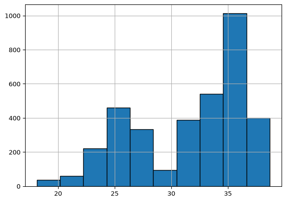
For the second option, we can call the hist() method directly on the column we want to visualize. This approach is often more straightforward when focusing on a single variable.
df["money"].hist(bins=10, edgecolor="black")
Histograms in Matplotlib
The pandas plot can be very convenient for quick visualizations, but it does not offer the same level of customization as Matplotlib. For more control over the appearance of your histogram, you can use Matplotlib’s plt.hist() function. This function allows you to customize various aspects of the histogram, such as the number of bins, colors, labels, and titles.
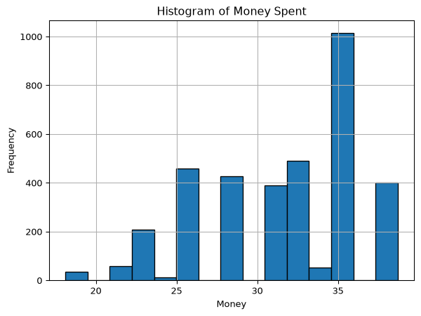
In the previous section, we arbitrarily decided to use 10 bins for our histogram. The number of bins can significantly affect the appearance and interpretability of the histogram. Too few bins can oversimplify the data, while too many bins can create a noisy representation. It’s better to calculate our bins mathematically. There are many ways to do this, but a common method is to use the cube root of the number of data points. This method provides a good balance between detail and clarity. We can do that simply by calling the count() method on our column and raising it to the power of one-third (**(1/3)).
import matplotlib.pyplot as pltplt.figure()plt.hist(df["money"], bins=int(df["money"].count() ** (1/3)), edgecolor="black")plt.title("Histogram of Money Spent")plt.xlabel("Money")plt.ylabel("Frequency")plt.grid()plt.show()
Histograms with Seaborn
Seaborn is a powerful visualization library built on top of Matplotlib that provides a high-level interface for creating attractive and informative statistical graphics. Moreover, it integrates well with pandas DataFrames, making it easy to visualize data directly from your DataFrame.
To move forward, you need to install Seaborn if you haven’t already. You can do this using uv from the command line:
uv add seaborn
Once you have Seaborn installed, we will first import it with the common alias of sns: import seaborn as sns. After that, we can create a histogram using the sns.histplot() function. This function provides a simple way to create histograms with additional features like kernel density estimation (KDE) and rug plots.
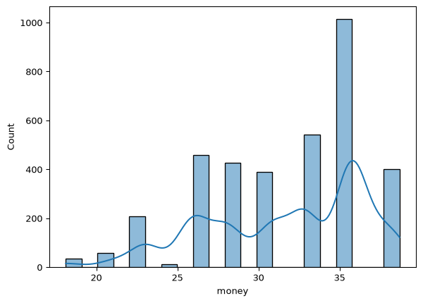
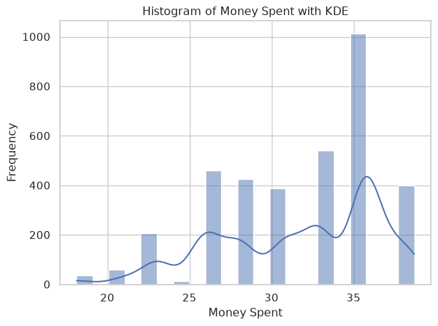
Since seaborn is built with pandas in mind, we can pass the entire DataFrame to the data argument and specify the column we want to visualize using the x argument. Additionally, we can enable the KDE overlay by setting the kde argument to True, which adds a smooth curve representing the estimated density of the data.
import seaborn as snsplt.figure()sns.histplot(data=df, x="money", kde=True )
The KDE line is a kernel density estimate, which is a way to estimate the probability density function of a continuous random variable. It provides a smooth curve that represents the distribution of the data, making it easier to visualize the underlying patterns and trends.
To make this figure more informative and pretty, we can set a theme using sns.set_theme(), and we can also add labels and a title to the plot using plt.xlabel(), plt.ylabel(), and plt.title(). As you can see, Seaborn adds onto Matplotlib, so we can still use Matplotlib functions to customize our plots.
plt.figure()sns.set_theme(style="whitegrid")sns.histplot(data=df, x="money", kde=True)plt.xlabel("Money Spent")plt.ylabel("Frequency")plt.title("Histogram of Money Spent with KDE")plt.show()
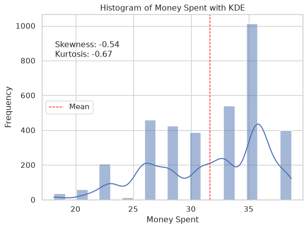
But this isn’t really enough. Why don’t we add more information to this visualization by adding text with the skew and kurtosis of the data? We can calculate these statistics using the scipy.stats library that we used in the previous chapter. In addition, we can add the mean line to the histogram using plt.axvline() and pass the mean_value as the x argument as well as set the color, linestyle, and linewidth. Finally, we can add a label to the mean line using the label argument and display the legend using plt.legend().
from scipy import statsskewness = stats.skew(df["money"])kurtosis = stats.kurtosis(df["money"])mean_value = df["money"].mean()string =f"""Skewness: {skewness:.2f}Kurtosis: {kurtosis:.2f}"""plt.figure()sns.set_theme(style="whitegrid")sns.histplot(data=df, x="money", kde=True)plt.xlabel("Money Spent")plt.ylabel("Frequency")plt.title("Histogram of Money Spent with KDE")plt.axvline(mean_value, color="red", linestyle="dashed", linewidth=1, label="Mean")plt.text(0.05,0.72, string, transform=plt.gca().transAxes, fontsize=12,)plt.legend()plt.show()