We will use this dataset form Kaggle.com that I have made available on my GitHub page: https://raw.githubusercontent.com/nkmwicz/data-for-students/refs/heads/main/soccer-players.csv
This data has information on players from transfermarkt.com. It specifically, has information on the birthdates of professional soccer players. There is a theory that exists that players born in the earlier months of the year are significantly more likely to play professional soccer than those born later. Theoretically, if all birth months have an equal chance at making the pros, there should be an even distribution of birth months. We will test this theory using the data.
First, let’s load the data and take a look at it.
import pandas as pd# Load the dataurl ="https://raw.githubusercontent.com/nkmwicz/data-for-students/refs/heads/main/soccer-players.csv"players = pd.read_csv(url)players.head()
player_id
first_name
last_name
name
last_season
current_club_id
player_code
country_of_birth
city_of_birth
country_of_citizenship
...
foot
height_in_cm
contract_expiration_date
agent_name
image_url
url
current_club_domestic_competition_id
current_club_name
market_value_in_eur
highest_market_value_in_eur
0
10
Miroslav
Klose
Miroslav Klose
2015
398
miroslav-klose
Poland
Opole
Germany
...
right
184.0
NaN
ASBW Sport Marketing
https://img.a.transfermarkt.technology/portrai...
https://www.transfermarkt.co.uk/miroslav-klose...
IT1
Società Sportiva Lazio S.p.A.
1000000.0
30000000.0
1
26
Roman
Weidenfeller
Roman Weidenfeller
2017
16
roman-weidenfeller
Germany
Diez
Germany
...
left
190.0
NaN
Neubauer 13 GmbH
https://img.a.transfermarkt.technology/portrai...
https://www.transfermarkt.co.uk/roman-weidenfe...
L1
Borussia Dortmund
750000.0
8000000.0
2
65
Dimitar
Berbatov
Dimitar Berbatov
2015
1091
dimitar-berbatov
Bulgaria
Blagoevgrad
Bulgaria
...
NaN
NaN
NaN
CSKA-AS-23 Ltd.
https://img.a.transfermarkt.technology/portrai...
https://www.transfermarkt.co.uk/dimitar-berbat...
GR1
Panthessalonikios Athlitikos Omilos Konstantin...
1000000.0
34500000.0
3
77
NaN
Lúcio
Lúcio
2012
506
lucio
Brazil
Brasília
Brazil
...
NaN
NaN
NaN
NaN
https://img.a.transfermarkt.technology/portrai...
https://www.transfermarkt.co.uk/lucio/profil/s...
IT1
Juventus Football Club
200000.0
24500000.0
4
80
Tom
Starke
Tom Starke
2017
27
tom-starke
East Germany (GDR)
Freital
Germany
...
right
194.0
NaN
IFM
https://img.a.transfermarkt.technology/portrai...
https://www.transfermarkt.co.uk/tom-starke/pro...
L1
FC Bayern München
100000.0
3000000.0
5 rows × 23 columns
Now, there are a lot of columns in this dataset that are unnecessary, so lets drop them (such as first_name, last_name, contract_expiration_date, image, etc.)
Now, let’s clean the date of birth to get birth months. We can do this by using the datetime methods of Pandas.
from datetime import datetimeplayers.dropna(subset=["date_of_birth"], inplace=True)players["birth_mth"] = pd.to_datetime(players["date_of_birth"]).dt.monthplayers.describe()
player_id
last_season
height_in_cm
market_value_in_eur
birth_mth
count
3.235600e+04
32356.000000
30023.000000
3.083700e+04
32356.00000
mean
3.446263e+05
2019.342533
182.291143
1.612785e+06
5.72648
std
2.806483e+05
3.965010
6.972046
6.365154e+06
3.42123
min
1.000000e+01
2012.000000
17.000000
1.000000e+04
1.00000
25%
1.069858e+05
2016.000000
178.000000
1.000000e+05
3.00000
50%
2.824215e+05
2020.000000
183.000000
2.500000e+05
5.00000
75%
5.241980e+05
2023.000000
187.000000
7.000000e+05
9.00000
max
1.309800e+06
2024.000000
207.000000
2.000000e+08
12.00000
We can also call many of these functions on their own just by using the mean(), median(), mode(), std(), min(), and max() functions. This time, let’s look at players’ heights.
We can also call many of these functions on their own just by using the mean(), median(), mode(), std(), min(), and max() functions. This time, let’s look at players’ heights.
Now let’s look at some other columns in the dataset that are categorical. We can loop over the columns checking of each on is numerical or not. To check if numerical we can use the pd.api.types.is_numeric_dtype() function.
for col in players.columns:ifnot pd.api.types.is_numeric_dtype(players[col]):print(f"{col}: {players[col].nunique()}")
Let’s find the different boundaries or thresholds of the data. For instance, what is the boundary separating the lower 25% and lower 30% from the rest of the data. We can use the quantile() function to find this.
# Find the 25th and 33rd percentilesq25 = players["height_in_cm"].dropna().quantile(0.25) *0.0328# to get feetq33 = players["birth_mth"].quantile(0.33)print(q25)print(q33)
5.838400000000001
3.0
We can also check the skew number of the data. This is a measure of the asymmetry of the data. A skew of 0 means the data is symmetrical. A positive skew means the data is skewed to the right, while a negative skew means the data is skewed to the left. While we are at it, let’s check the kurtosis as well.
The skewness output is 0.2620. This is a slightly positive skewness score which means the data is slightly skewed to the right.
The kurtosis score is -1.1306 which means the data is fairly flat. This means the data is slightly less peaked than a normal distribution.
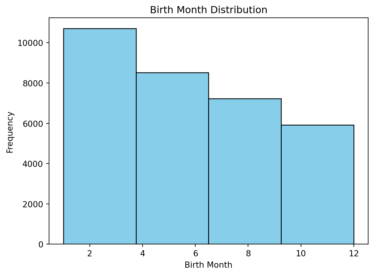
import matplotlib.pyplot as pltplt.hist(players["birth_mth"], bins=4, color="skyblue", edgecolor="black")plt.xlabel("Birth Month")plt.ylabel("Frequency")plt.title("Birth Month Distribution")plt.show()
The nature of birth months is that we expect an equal distribution of birth months. However, the data shows that there are more players born in the earlier months of the year. This is consistent with the theory that players born in the earlier months of the year are more likely to play professional soccer. In fact, is a dramatic difference in the number of players born in the earlier months compared to the later months.
for i, num inenumerate(players["birth_mth"].value_counts()):print(f"Month {i+1}: {num} or {num/players.shape[0]*100:.2f}%")
Month 1: 4066 or 12.57%
Month 2: 3376 or 10.43%
Month 3: 3256 or 10.06%
Month 4: 3001 or 9.27%
Month 5: 2915 or 9.01%
Month 6: 2595 or 8.02%
Month 7: 2534 or 7.83%
Month 8: 2400 or 7.42%
Month 9: 2294 or 7.09%
Month 10: 2104 or 6.50%
Month 11: 1973 or 6.10%
Month 12: 1842 or 5.69%