The primary way to visualize numerical to numerical data is with a scatter plot. Scatter plots show the relationship between two numerical variables by plotting data points on a two-dimensional graph, where each axis represents one of the variables.
To begin with, let’s look at our penguin dataset from the last chapter.
import pandas as pdurl ="https://raw.githubusercontent.com/dataprofessor/data/refs/heads/master/penguins_cleaned.csv"penguins = pd.read_csv(url)penguins.head()
species
island
bill_length_mm
bill_depth_mm
flipper_length_mm
body_mass_g
sex
0
Adelie
Torgersen
39.1
18.7
181
3750
male
1
Adelie
Torgersen
39.5
17.4
186
3800
female
2
Adelie
Torgersen
40.3
18.0
195
3250
female
3
Adelie
Torgersen
36.7
19.3
193
3450
female
4
Adelie
Torgersen
39.3
20.6
190
3650
male
When we represent a bivariate numerical-to-numerical relationship with a scatter plot, each point on the plot corresponds to an observation in the dataset. The position of the point along the x-axis represents the value of one numerical variable, while the position along the y-axis represents the value of the other numerical variable. This allows us to visually assess patterns, trends, and potential correlations between the two variables.
Scatter Plots with Matplotlib
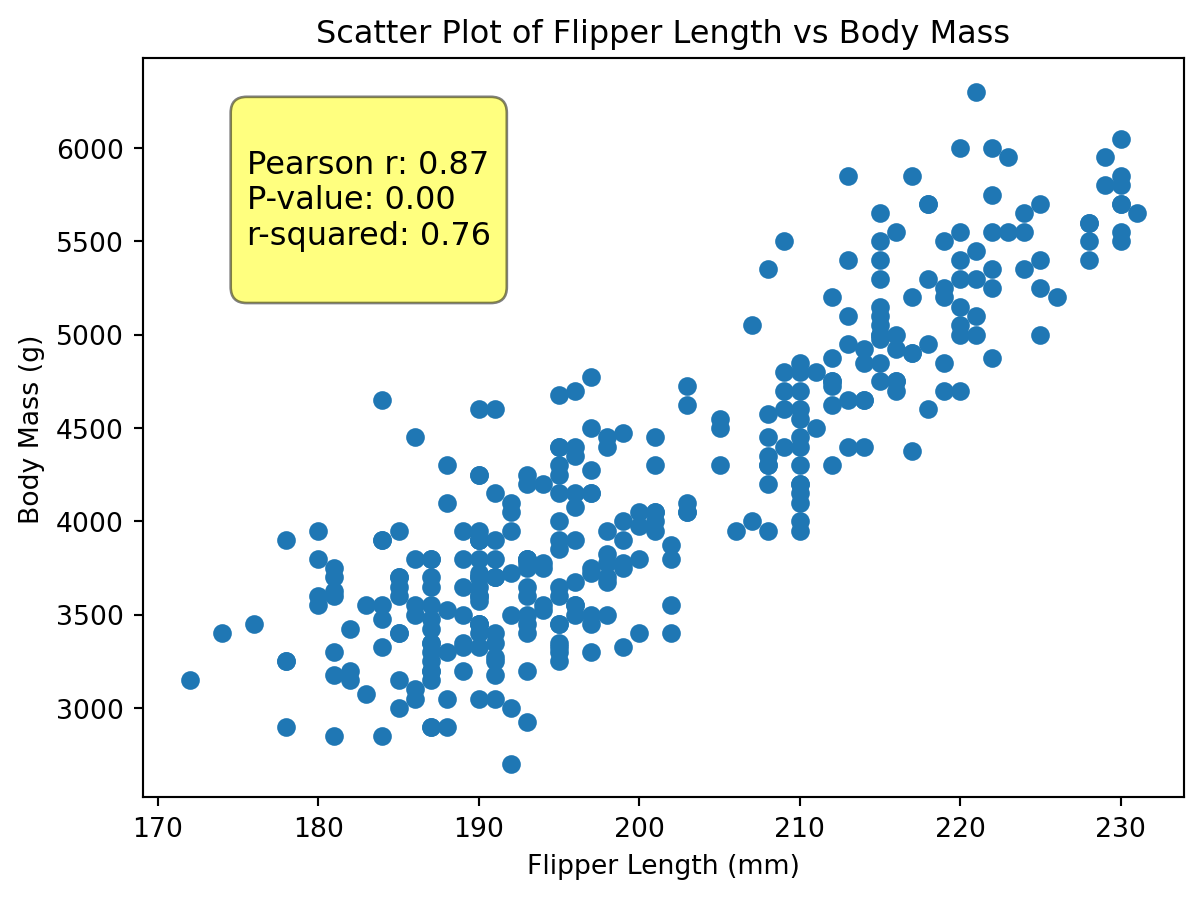
Let’s first get acquainted with scatter plots using the matplotlib library. We will create a scatter plot to visualize the relationship between flipper_length_mm and body_mass_g.
matplotlib makes it particularly easy to create a scatter plot. We only need to call the scatter method and provide the x and y variables.
import matplotlib.pyplot as pltfrom scipy import statsr, p = stats.pearsonr(penguins["flipper_length_mm"], penguins["body_mass_g"])text =f"""Pearson r: {r:.2f}P-value: {p:.2f}r-squared: {r**2:.2f}"""plt.figure(figsize=(7, 5))plt.scatter(x=penguins["flipper_length_mm"], y=penguins["body_mass_g"])plt.title("Scatter Plot of Flipper Length vs Body Mass")plt.xlabel("Flipper Length (mm)")plt.ylabel("Body Mass (g)")plt.text(0.10,0.70, text, transform=plt.gca().transAxes, fontsize=12, bbox=dict(boxstyle="round,pad=0.5", fc="yellow", alpha=0.5),)plt.show()
We can see from the scatter plot alone that there appears to be a positive correlation between the flipper length and body mass of penguins. As the flipper length increases, the body mass tends to increase as well. This visual representation helps us understand the relationship between these two numerical variables. When we add the Pearson correlation coefficient (r) and p-value to the plot, we can quantify this relationship. The r value of approximately 0.87 indicates a strong positive linear relationship, while the very small p-value suggests that this correlation is statistically significant.
matplotlib provides other customization options for our text as is clear in the above codeblock. We can change fontsize, but we can also create a style for the bounding box (bbox) that contains the text. In this case, we created a rounded box with some padding, a yellow background color (fc), and set the transparency with alpha. Finally, we set the boxstyle to round,pad=0.5 to create rounded corners with some padding around the text.
Scatter Plots with Seaborn
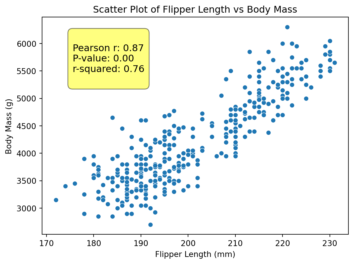
Seaborn makes scatter plots even easier by providing a high-level interface for drawing attractive and informative statistical graphics. We can use the scatterplot function from the seaborn library to create a scatter plot of the same variables.
We can do the same thing as above, but with less code and in a more descriptive manner because seaborn works directly with pandas DataFrames. Moreover, seaborn automatically adds some nice styling to the plots, making them visually appealing with minimal effort. As chapter 10 discussed, seaborn works well as declared variables. In this way, we can set the title and axis labels using the set method. The set method allows us to customize various aspects of the plot, such as the title and axis labels, in a clean and organized manner.
import seaborn as snsplt.figure(figsize=(7, 5))scat = sns.scatterplot(data=penguins, x="flipper_length_mm", y="body_mass_g")scat.set( title="Scatter Plot of Flipper Length vs Body Mass", xlabel="Flipper Length (mm)", ylabel="Body Mass (g)",)scat.text(0.10,0.70, text, transform=scat.transAxes, fontsize=12, bbox=dict(boxstyle="round,pad=0.5", fc="yellow", alpha=0.5),)plt.show()