11.3 Scatter Plots and More

Bivariate N2N Visualizations

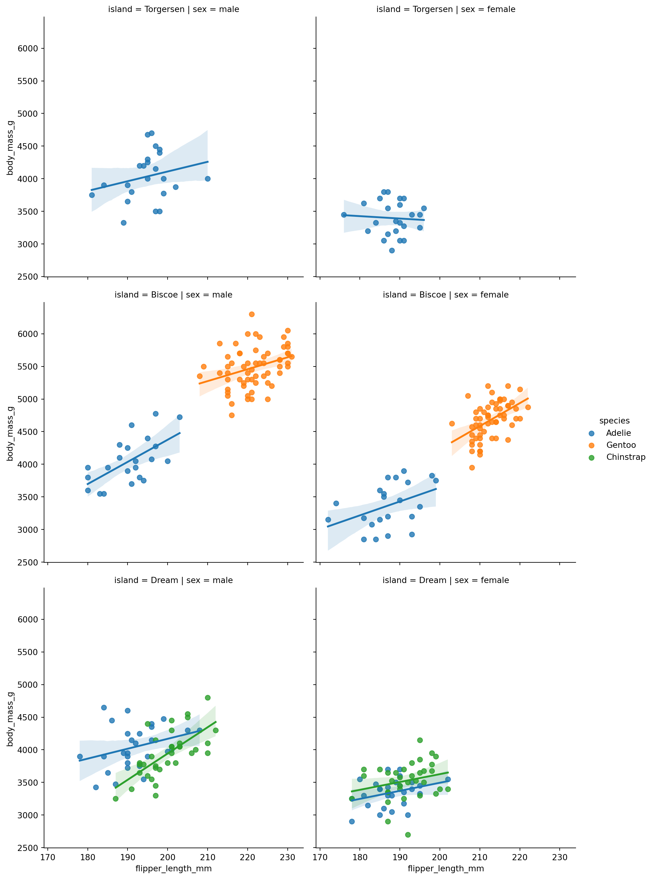
We can also create scatter plots combined with other plots. One of the easiest ways to do this is the lmplot method from seaborn, we can use it to create multiple plots with regression lines.

import pandas as pd
import matplotlib.pyplot as plt
import seaborn as sns

url = "https://raw.githubusercontent.com/dataprofessor/data/refs/heads/master/penguins_cleaned.csv"
penguins = pd.read_csv(url)
penguins.head()

	species	island	bill_length_mm	bill_depth_mm	flipper_length_mm	body_mass_g	sex
0	Adelie	Torgersen	39.1	18.7	181	3750	male
1	Adelie	Torgersen	39.5	17.4	186	3800	female
2	Adelie	Torgersen	40.3	18.0	195	3250	female
3	Adelie	Torgersen	36.7	19.3	193	3450	female
4	Adelie	Torgersen	39.3	20.6	190	3650	male

sns.lmplot(
    x="flipper_length_mm",
    y="body_mass_g",
    hue="species",
    data=penguins,
    col="sex",
    row="island",
)

This figure plots the different species of penguins in different colors, separated by sex (columns) and island (rows). Each subplot contains a scatter plot of flipper length vs body mass, along with a regression line for each species.

We can also create joint plots withe seaborn that combine scatter plots with histograms or density plots.

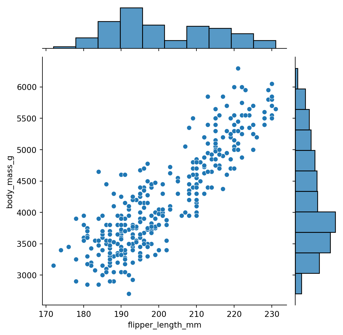
sns.jointplot(
    x="flipper_length_mm",
    y="body_mass_g",
    data=penguins,
)

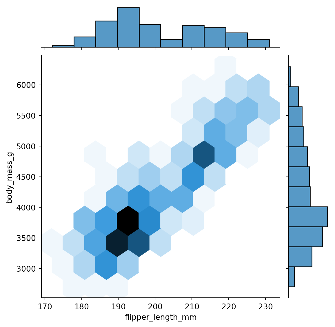
We can also change the kind of plot used in the joint plot. For example, we can use a hexbin plot to visualize the density of points.

sns.jointplot(
    x="flipper_length_mm",
    y="body_mass_g",
    data=penguins,
    kind="hex",
)

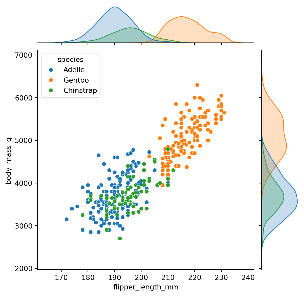
We can also color the points by species using the hue parameter.

sns.jointplot(
    x="flipper_length_mm",
    y="body_mass_g",
    data=penguins,
    kind="scatter",
    hue="species",
)

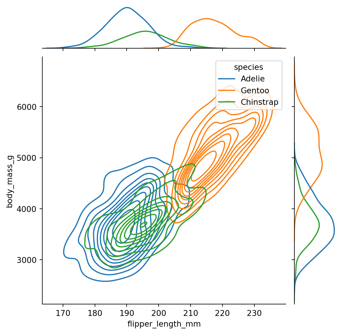
Finally, we can create a kernel density estimate (KDE) plot to visualize the distribution of points.

sns.jointplot(
    x="flipper_length_mm",
    y="body_mass_g",
    data=penguins,
    kind="kde",
    hue="species",
)