9.3 Box Plots

Univariate Visualizations

While histograms are great for understanding the distribution of a dataset, box plots (or box-and-whisker plots) provide a concise summary of the data’s key statistics, including its median, quartiles, and potential outliers. They are particularly useful for comparing distributions across different categories or groups.

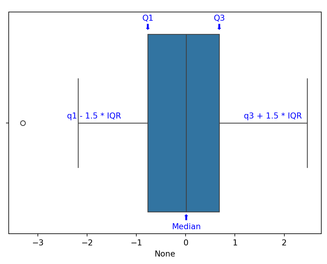
First let’s learn how to read a box plot:

The main box represents the interquartile range (IQR), which contains the middle 50% of the data.
1. The IQR is calculated as Quartile3 (q3) - Quartile1 (q1).
The middle line in the box indicates the median (Quartile2) of the dataset.
The “whiskers” extend from the box to the smallest and largest values within 1.5 * IQR from q1 and q3, respectively.
Data points outside this range are considered outliers and are often represented as individual dots.

A box plot provides a visual summary of the distribution of the dataset, highlighting its central tendency, variability, and potential outliers. This makes it a powerful tool for exploratory data analysis and comparison across different groups or categories.

Box Plots with Matplotlib

To begin building our box plot, we will first import our data from the same dataset we used for our histogram example.

import matplotlib.pyplot as plt
import pandas as pd

df = pd.read_csv("coffee_sales.csv")
df.head()

	hour_of_day	cash_type	money	coffee_name	Time_of_Day	Weekday	Month_name	Weekdaysort	Monthsort	Date	Time
0	10	card	38.7	Latte	Morning	Fri	Mar	5	3	2024-03-01	10:15:50.520000
1	12	card	38.7	Hot Chocolate	Afternoon	Fri	Mar	5	3	2024-03-01	12:19:22.539000
2	12	card	38.7	Hot Chocolate	Afternoon	Fri	Mar	5	3	2024-03-01	12:20:18.089000
3	13	card	28.9	Americano	Afternoon	Fri	Mar	5	3	2024-03-01	13:46:33.006000
4	13	card	38.7	Latte	Afternoon	Fri	Mar	5	3	2024-03-01	13:48:14.626000

Building a box plot with Matplotlib is straightforward using the boxplot function. Here’s how to create a basic box plot:

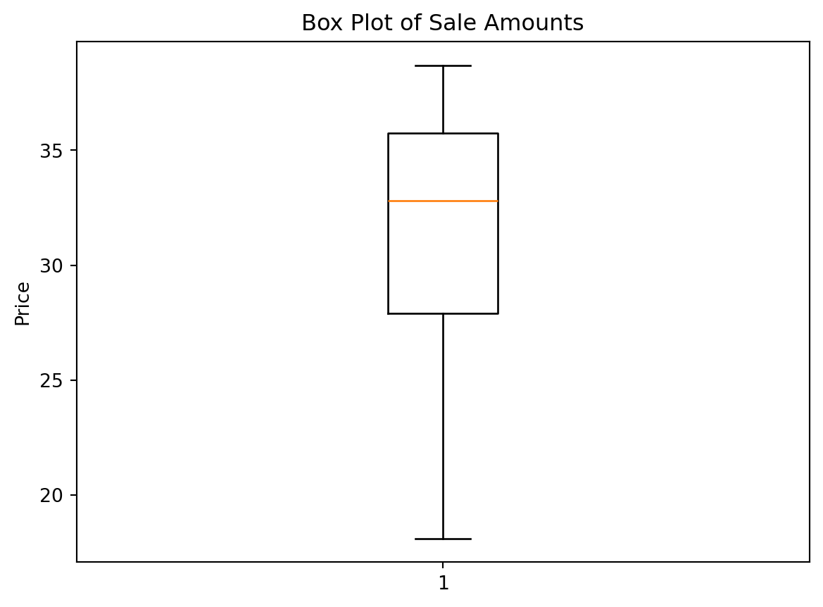
Now we can also change the orientation of the box plot to be horizontal instead of vertical. This can be done by using the vert parameter and setting it to False. We can also update the x-tick label—the one below the box—to be “Money” instead of “1”.

plt.boxplot(df["money"], vert=False)
plt.xlabel("Price")
plt.yticks([1], ["Money"])
plt.title("Box Plot of Sale Amounts")
plt.show()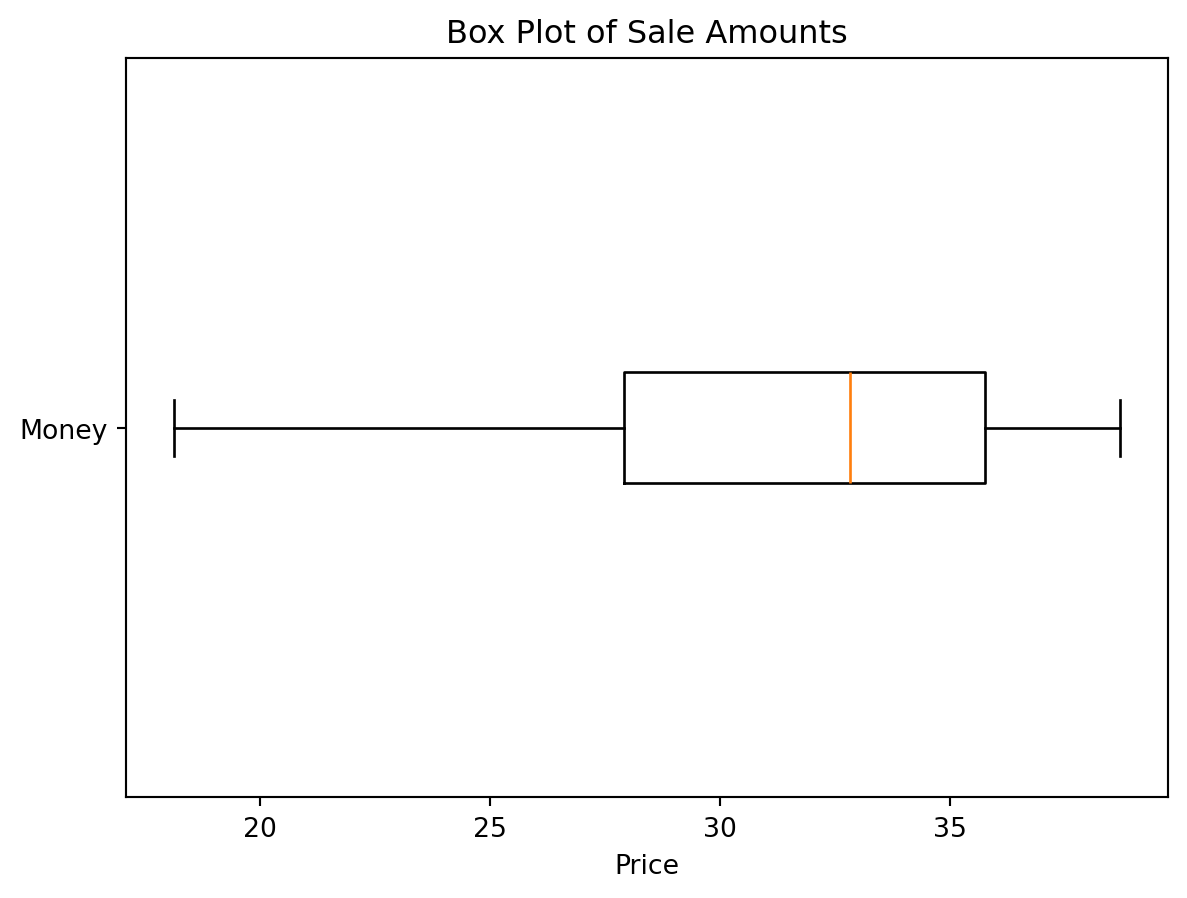

Notice, that the yticks() method takes two arguments: the first is a list of positions to place the ticks, and the second is a list of labels to use at those positions. Since we only have one box, we only need one position and one label.

Box Plots with Seaborn

Seaborn provides a more aesthetically pleasing and feature-rich way to create box plots. The boxplot function in Seaborn is versatile and allows for easy customization. Here’s how to create a box plot using Seaborn:

import seaborn as sns

sns.boxplot(x=df["money"], color="lightblue")
plt.xlabel("Price")
plt.title("Box Plot of Sale Amounts")
plt.show()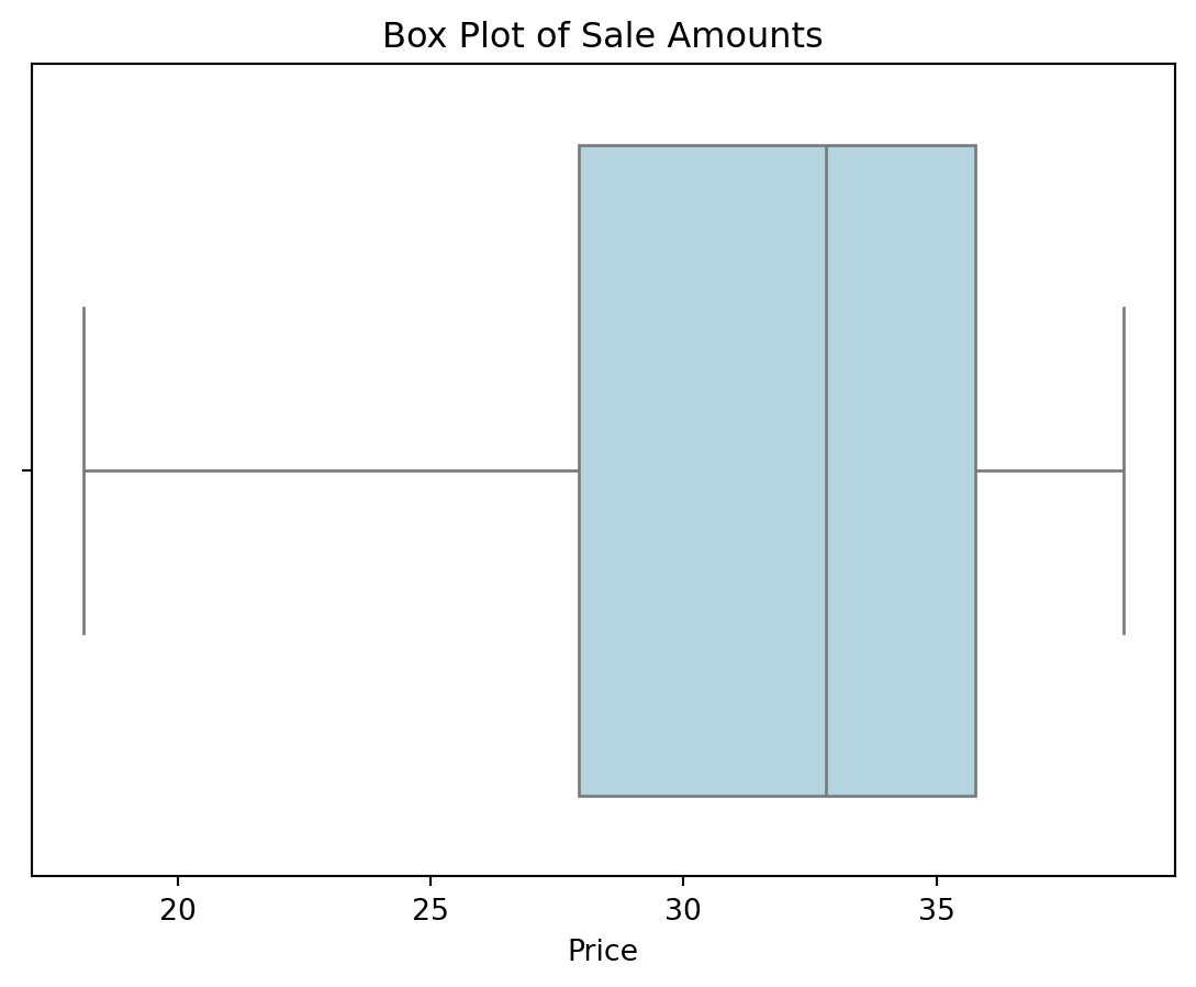

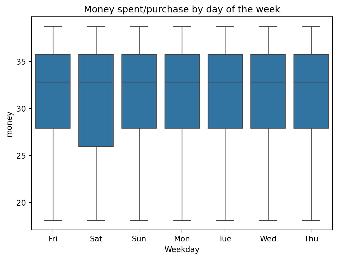
If we remember that seaborn is built on top of pandas, we can also pass in a DataFrame and specify the column we want to plot using the x parameter, then we can also specify the y parameter if we want to view multiple box plots divided by a categorical variable. For instance, if we wanted to see how the sale amounts differ by the day of the week, we could do the following:

cat_boxes = sns.boxplot(data=df, x="Weekday", y="money")
plt.title("Money spent/purchase by day of the week")
plt.show()