from seaborn import load_dataset
import pandas as pd

df = load_dataset("titanic")

print(f"var = {df['age'].var()}")
print(f"st.dev = {df['age'].std()}")
var = 211.01912474630802
st.dev = 14.526497332334042Univariate Statistics
Now that we have understood measures of central tendency, let’s explore measures of variance and shapes of distributions. These can help us understand how “normal” or “gaussian” our data is. To understand variance, we will look at variance and standard deviation, which are measures of spread. To understand the shape of distributions, we will look at skewness and kurtosis.
Variance and standard deviation measure how much the average data point deviates from the mean. A low variance indicates that data points are close to the mean, while a high variance indicates that data points are spread out over a wider range. The two are strongly related, as standard deviation is simply the square root of variance. Let’s look at the formulas for both:
\[\text{Variance} (\sigma^2) = \frac{\sum (x_i - \mu)^2}{N}\]
Where:
\[\text{Standard Deviation} (\sigma) = \sqrt{\text{Variance}} = \sqrt{\frac{\sum (x_i - \mu)^2}{N}}\]
Where:
Both of these equations measure the variance and standard deviation of a population. A population includes all members of a specified group. For example, if you were studying the heights of all students in a school, the population would include every single student in that school. Rarely in practice do we have access to data for an entire population. More often, we work with samples, which are subsets of the population. When calculating variance and standard deviation for a sample, we use slightly different formulas to account for the fact that we are working with a subset of the population. The formulas for sample variance and sample standard deviation are as follows:
\[\text{Sample Variance} (s^2) = \frac{\sum (x_i - \bar{x})^2}{n - 1}\]
Where:
\[\text{Sample Standard Deviation} (s) = \sqrt{\text{Sample Variance}} = \sqrt{\frac{\sum (x_i - \bar{x})^2}{n - 1}}\]
Where:
Effectively, when we are calculating these statistics for a sample, we subtract the number of data points by 1 (n - 1) instead of using the total number of data points (N). This adjustment is known as Bessel’s correction and helps to provide a more accurate estimate of the population variance and standard deviation from a sample. Because we will frequently perform our calculations on samples, most of our tooling will default to the sample formulas. If we, however, have access to the entire population, we can specify that in our calculations.
Now let’s explore what variance and standard deviation are actually doing. For each data point, we are calculating the difference between the data point and the mean. Because we will have data points on both sides of the mean, we square the differences to ensure that all values are positive. We then sum these squared differences and divide by the number of data points (or number of data points minus one for samples) to get the average squared difference from the mean. This gives us the variance. Variance is usually difficult to interpret because it is in squared units. The standard deviation is simply the square root of the variance, which brings it back to the original units of measurement.
TLDR: Variance and standard deviation measure the average distance of all data points from the mean. A low variance or standard deviation indicates that data points are close to the mean, while a high variance or standard deviation indicates that data points are spread out over a wider range.
Fortunately, in Python and Pandas, we can easily calculate variance and standard deviation using built-in functions. In Pandas, we can simply use the .var() and .std() methods on a DataFrame or Series. Let’s look at an example using a sample dataset:
from seaborn import load_dataset
import pandas as pd
df = load_dataset("titanic")
print(f"var = {df['age'].var()}")
print(f"st.dev = {df['age'].std()}")var = 211.01912474630802
st.dev = 14.526497332334042This will give us the variance and standard deviation of the age column in the Titanic dataset. By default, these methods calculate the sample variance and sample standard deviation. If we wanted to calculate the population variance and population standard deviation, we could pass the parameter ddof=0 to the methods. ddof stands for “delta degrees of freedom” and is used to adjust the divisor in the calculation. By default, ddof=1, which calculates the sample variance and sample standard deviation. Setting ddof=0 calculates the population variance and population standard deviation.
Notice here, that the standard deviation calculation provides a more interpretable number, as it is in the same units as the original data (years, in this case). The variance, on the other hand, is in squared units (years squared), which can be harder to interpret.
We can similarly calculate variance and standard deviation for all numerical columns in a DataFrame by simply calling the methods on the entire DataFrame:
print(df.var(numeric_only=True))
print(df.std(numeric_only=True))
survived 0.236772
pclass 0.699015
age 211.019125
sibsp 1.216043
parch 0.649728
fare 2469.436846
adult_male 0.239723
alone 0.239723
dtype: float64
survived 0.486592
pclass 0.836071
age 14.526497
sibsp 1.102743
parch 0.806057
fare 49.693429
adult_male 0.489615
alone 0.489615
dtype: float64We pass in numeric_only=True to ensure that we are only calculating these statistics for numerical columns, as variance and standard deviation are not defined for categorical data.
Skewness and kurtosis are measures that describe the shape of a distribution. Skewness measures the asymmetry of the distribution, while kurtosis measures the “tailedness” or the presence of outliers in the distribution.
In short skewness measures how much of the data is on either side of the mean. A perfectly symmetrical distribution will have a skewness of 0. If the distribution has a longer tail on the right side (positive skew), it will have a positive skewness value. Another way to think of this is if more data exists on the positive side of the mean. Conversely, if the distribution has a longer tail on the left side (negative skew), it will have a negative skewness value. Or if more data exists on the negative side of the mean.
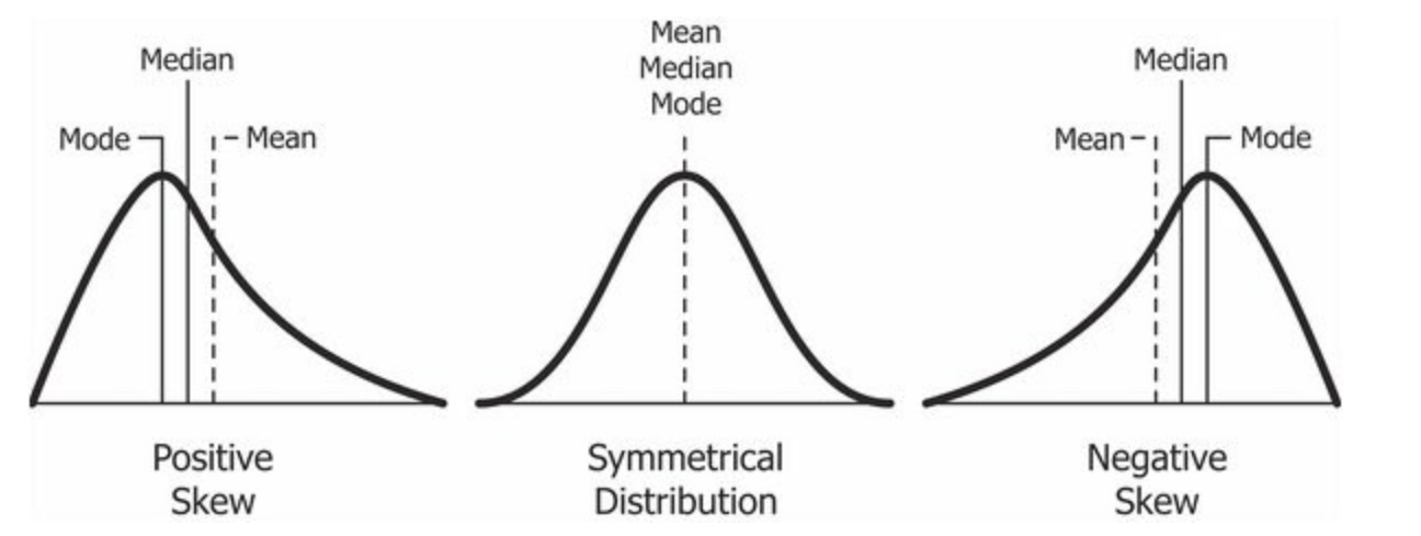
Skewness can be calculated using the following formula:
\[\text{Skewness} = \frac{N}{(N-1)(N-2)} \sum \left(\frac{x_i - \bar{x}}{s}\right)^3\]
Where:
In Python and Pandas, we can easily calculate skewness using the built-in .skew() method on a DataFrame or Series. Let’s look at an example using the Titanic dataset:
print(df['age'].skew())0.38910778230082704This will give us the skewness of the age column in the Titanic dataset. A positive value indicates a right-skewed distribution, while a negative value indicates a left-skewed distribution.
Since the skewness of a normal distribution is 0, we can use skewness to assess how closely our data follows a normal distribution. As general guidelines:
We can similarly calculate skewness for all numerical columns in a DataFrame by simply calling the method on the entire DataFrame:
print(df.skew(numeric_only=True))survived 0.478523
pclass -0.630548
age 0.389108
sibsp 3.695352
parch 2.749117
fare 4.787317
adult_male -0.420431
alone -0.420431
dtype: float64Once again, we pass in numeric_only=True to ensure that we are only calculating this statistic for numerical columns.
Finally, we can also use the scipy.stats library to calculate skewness. You can install it using uv if you haven’t already or the anaconda navigator.
from scipy import stats
print(stats.skew(df["age"], nan_policy="omit"))0.38828985146986567Kurtosis measures the “tailedness” of a distribution, or how heavy or light the tails are compared to a normal distribution. A normal distribution has a kurtosis of 3. Distributions with kurtosis greater than 3 are called leptokurtic and have heavier tails, indicating a higher likelihood of extreme values (outliers). Distributions with kurtosis less than 3 are called platykurtic and have lighter tails, indicating fewer extreme values.
print(df['age'].kurt())0.17827415364210353Pandas uses the Fisher definition of kurtosis, which subtracts 3 from the result to provide excess kurtosis. Therefore, a normal distribution will have an excess kurtosis of 0. A positive excess kurtosis indicates a leptokurtic distribution, while a negative excess kurtosis indicates a platykurtic distribution.
Kurtosis measurements make a few assumptions about the data, primarily that it is continuous and unbounded. This means that kurtosis is not well-suited for categorical data or data with natural bounds (e.g., percentages). Additionally, kurtosis can be sensitive to outliers, so it is important to consider the presence of extreme values in the data when interpreting kurtosis values.
We can also use the scipy.stats library to calculate kurtosis. You can install it using uv if you haven’t already or the anaconda navigator.
from scipy import stats

print(stats.kurtosis(df["age"], nan_policy="omit"))0.16863657224286044The nan_policy="omit" parameter ensures that any NaN values in the data are ignored when calculating kurtosis.