9.4 Multi Plots

Univariate Visualizations

We can also create multiple plots in a single figure to compare distributions or visualize different aspects of the same data. This is particularly useful for identifying patterns, trends, or anomalies across different subsets of data.

Let’s continue to work with our coffee sales dataset.

import matplotlib.pyplot as plt
import seaborn as sns
import pandas as pd

df = pd.read_csv("coffee_sales.csv")
df.head()

	hour_of_day	cash_type	money	coffee_name	Time_of_Day	Weekday	Month_name	Weekdaysort	Monthsort	Date	Time
0	10	card	38.7	Latte	Morning	Fri	Mar	5	3	2024-03-01	10:15:50.520000
1	12	card	38.7	Hot Chocolate	Afternoon	Fri	Mar	5	3	2024-03-01	12:19:22.539000
2	12	card	38.7	Hot Chocolate	Afternoon	Fri	Mar	5	3	2024-03-01	12:20:18.089000
3	13	card	28.9	Americano	Afternoon	Fri	Mar	5	3	2024-03-01	13:46:33.006000
4	13	card	38.7	Latte	Afternoon	Fri	Mar	5	3	2024-03-01	13:48:14.626000

The easiest way to create multiple plots is to use the subplots function from Matplotlib. This function allows us to create a grid of plots within a single figure.

plt.subplots() takes several arguments. nrows and ncols specify the number of rows and columns of subplots, respectively. The function returns a figure object and an array of axes objects that we can use to plot our data. Then we can also determine the relative size of each subplot using height_ratios and width_ratios. They both take in a list of integers that specify the relative size of each row or column.

# Create a figure with multiple subplots
fig, (ax1, ax2) = plt.subplots(nrows=2, ncols=1, height_ratios=[2, 8])
hist = sns.histplot(data=df, x="money", ax=ax2)
box = sns.boxplot(data=df, x="money", ax=ax1)
plt.show()

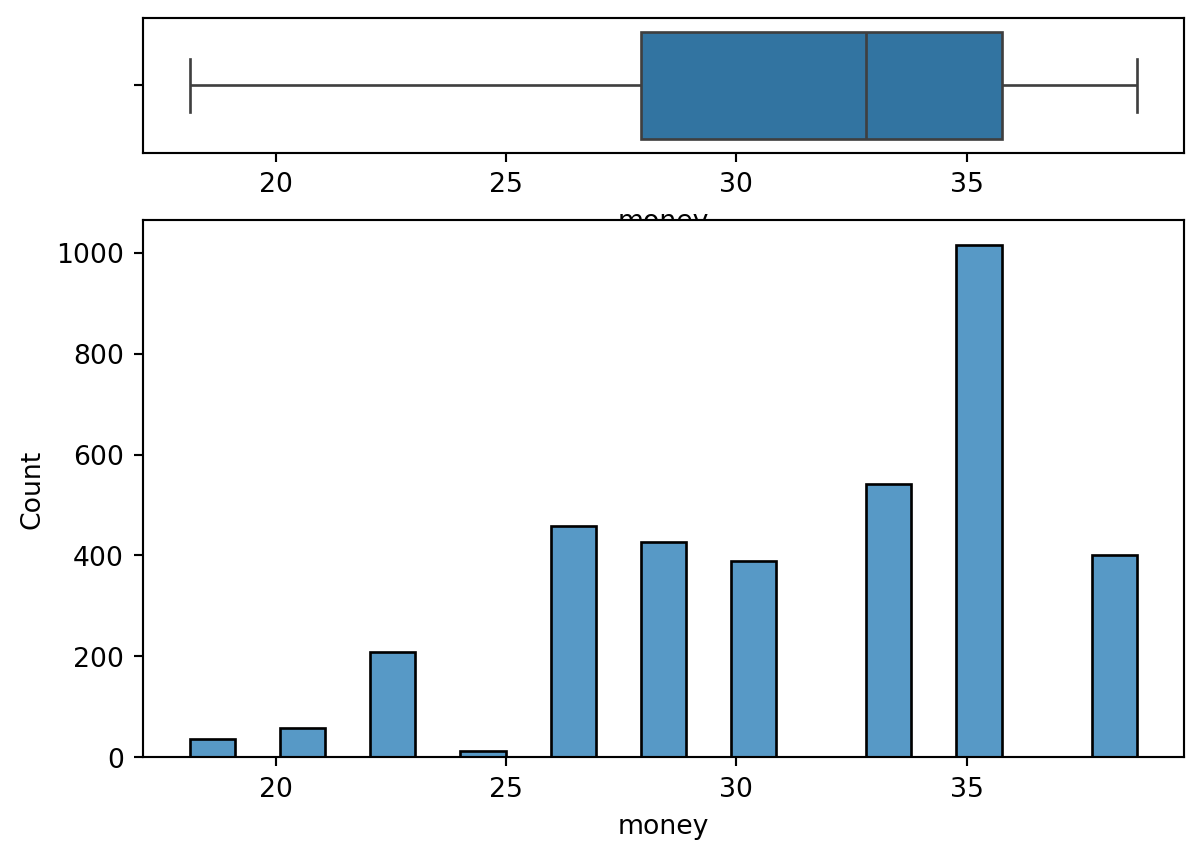
Notice, we now have two plots in a single figure. The box plot is on top and the histogram is on the bottom. We specified height_ratios=[2, 8] to make the histogram larger than the box plot. We set the hist on the second axis (ax2) and the box on the first axis (ax1), using the ax parameter in both Seaborn functions.

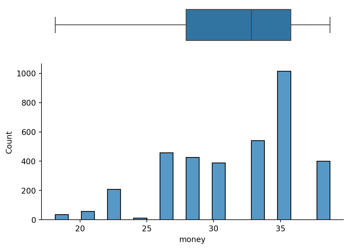
But we can improve this further. Since both plots are sharing the x-axis, we can remove the x-axis from the box to reduce clutter and remove the top and right axis from the hist for the same reason.

fig, (ax1, ax2) = plt.subplots(nrows=2, ncols=1, height_ratios=[2, 8])
hist = sns.histplot(data=df, x="money", ax=ax2)
box = sns.boxplot(data=df, x="money", ax=ax1)
box.set(xlabel="")  # Remove x-axis label from box plot
ax1.spines["bottom"].set_visible(False)  # Remove bottom spine from box plot
ax1.spines["top"].set_visible(False)  # Remove top spine from box plot
ax1.spines["right"].set_visible(False)  # Remove right spine from box plot
ax1.spines["left"].set_visible(False)  # Remove left spine from box plot
ax1.set(yticks=[])  # Remove y-ticks from box plot
ax1.set(xticks=[])  # Remove x-ticks from box plot
ax2.spines["top"].set_visible(False)  # Remove top spine from histogram
ax2.spines["right"].set_visible(False)  # Remove right spine from histogram
plt.show()

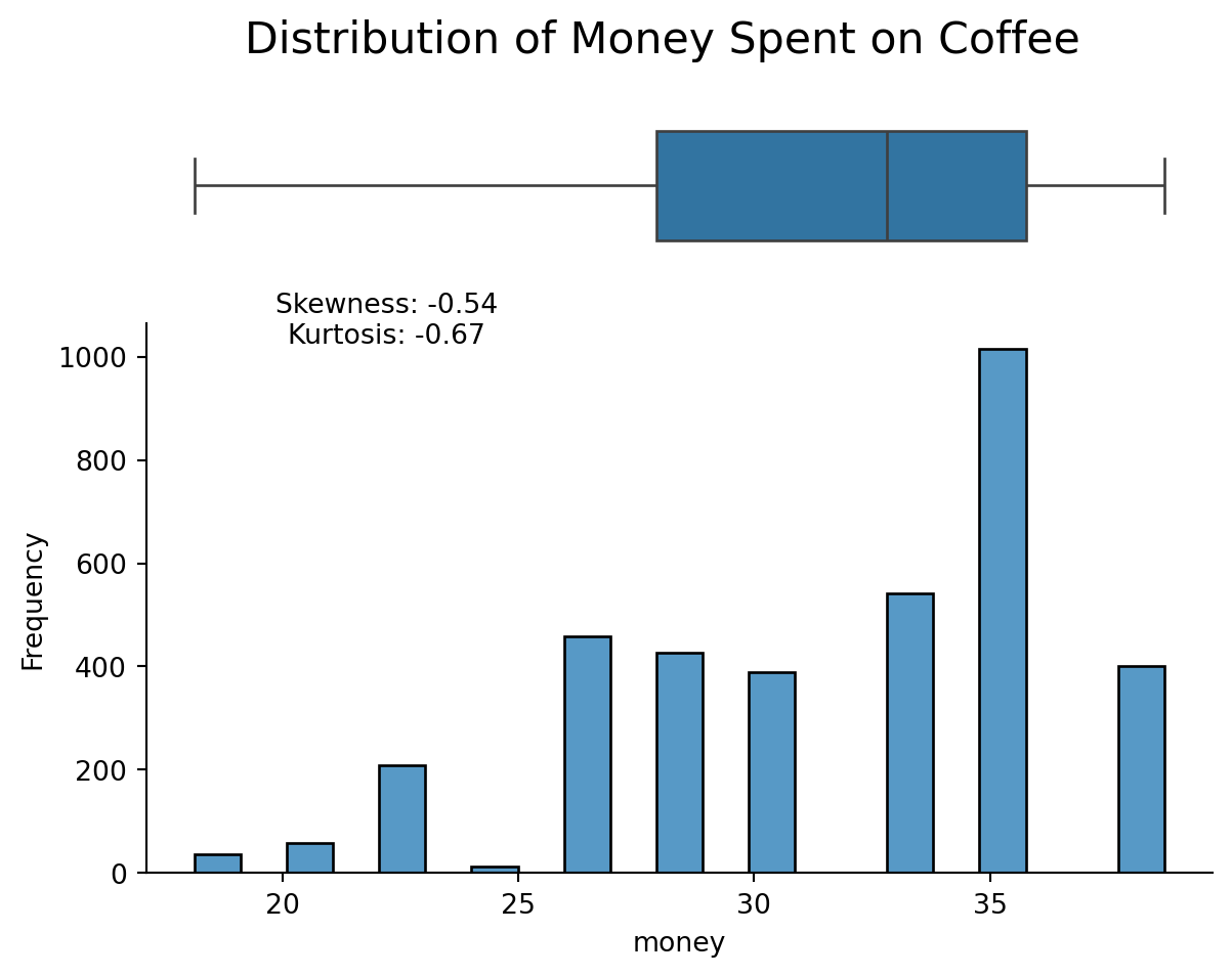
But we aren’t done yet. Because we need to add a title to the entire figure. We can also improve the y-label and add information on the skewness and kurtosis of the distribution. Because we have

from scipy.stats import skew, kurtosis

skewness = skew(df["money"], nan_policy="omit")
kurt = kurtosis(df["money"], nan_policy="omit")

fig, (ax1, ax2) = plt.subplots(nrows=2, ncols=1, height_ratios=[2, 8])
hist = sns.histplot(data=df, x="money", ax=ax2)
box = sns.boxplot(data=df, x="money", ax=ax1)
box.set(xlabel="")  # Remove x-axis label from box plot
ax1.spines["bottom"].set_visible(False)  # Remove bottom spine from box plot
ax1.spines["top"].set_visible(False)  # Remove top spine from box plot
ax1.spines["right"].set_visible(False)  # Remove right spine from box plot
ax1.spines["left"].set_visible(False)  # Remove left spine from box plot
ax1.set(yticks=[])  # Remove y-ticks from box plot
ax1.set(xticks=[])  # Remove x-ticks from box plot
ax2.spines["top"].set_visible(False)  # Remove top spine from histogram
ax2.spines["right"].set_visible(False)  # Remove right spine from histogram
ax2.set_ylabel("Frequency")  # Add y-axis label to histogram
plt.figtext(
    0.3,
    0.65,
    f"Skewness: {skewness:.2f}\nKurtosis: {kurt:.2f}",
    ha="center",
    fontsize=10,
    transform=fig.transFigure,
)
fig.suptitle("Distribution of Money Spent on Coffee", fontsize=16)
plt.show()

Notice, because we are working with subplots(), somethings are phrased differently. For example, to add a title to the entire figure, we use fig.suptitle() instead of plt.title(). To add a y-label to the histogram, we use ax2.set_ylabel() instead of plt.ylabel(). And to add text to the figure, we use plt.figtext() with the transform=fig.transFigure argument to position the text relative to the entire figure.