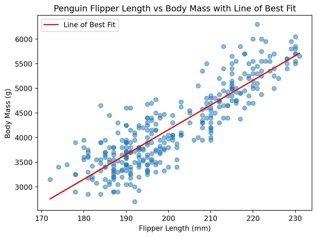
When we are plotting the relationship between two numerical variables, it is often helpful to add a line of best fit (also known as a regression line) to our scatter plot. This line represents the trend in the data and can help us understand the relationship between the two variables more clearly.
Adding a Line of Best Fit with Matplotlib
To add a line of best fit to our scatter plot using matplotlib, we can use the linregress function from the scipy.stats module to calculate the slope and intercept of the line. We can then use these values to plot the line on top of our scatter plot.
When we use the linregress function, it returns several values, including the slope and intercept of the line, as well as the correlation coefficient (r_value), p-value, and standard error. We can use the slope and intercept to create the line of best fit.
The equation of the line can be expressed as: y = mx + b, where m is the slope and b is the intercept.
slope: Also known as “m” in the equation of a line, it represents the rate of change of the dependent variable (y) with respect to the independent variable (x). As the independent variable (x) increases by one unit, the dependent variable (y) changes by the value of the slope (m). It is often interpreted as “rise over run.” Here it is represented as a decimal value. If m=0.2, for every 1 unit increase in x, y increases by 0.2 units.
intercept: Also known as “b” in the equation of a line, it represents the value of the dependent variable (y) when the independent variable (x) is equal to zero. It is the point where the line crosses the y-axis. The intercept provides a starting point for the line and helps to position it correctly on the graph.
When we calculate the points for each y-value, we can use the intercept to adjust the line vertically on the graph.
r_value: the correlation coefficient. We are already familiar with this value.
p_value: the p-value for the r value.
std_err: the standard error of the estimate. The standard quantifies the degree to which we would expect slope to vary from sample to sample in a similar way as the p-value calculates the likelihood of observing a slope as extreme as the one calculated if the null hypothesis were true.
In other words, we will calculate the y-values for each x-value in our dataset using the slope and intercept obtained from linregress.
import pandas as pdimport matplotlib.pyplot as pltfrom scipy import statsurl ="https://raw.githubusercontent.com/dataprofessor/data/refs/heads/master/penguins_cleaned.csv"penguins = pd.read_csv(url)slope, intercept, r_value, p_value, std_err = stats.linregress( penguins["flipper_length_mm"], penguins["body_mass_g"])plt.figure(figsize=(7, 5))plt.scatter(penguins["flipper_length_mm"], penguins["body_mass_g"], alpha=0.5)# Calculate the line of best fitline = slope * penguins["flipper_length_mm"] + intercept# Plot the line of best fitplt.plot(penguins["flipper_length_mm"], line, color="red", label="Line of Best Fit")plt.xlabel("Flipper Length (mm)")plt.ylabel("Body Mass (g)")plt.title("Penguin Flipper Length vs Body Mass with Line of Best Fit")plt.legend()plt.show()
To plot the line of best fit, we calculate the y-values for each x-value in our dataset using the slope and intercept obtained from linregress. For each x-value (flipper length), we multiply it by the slope and add the y-intercept (the value of y when x=0). The y-intercept helps to position the line correctly on the graph by adding any extra vertical offset. In other words, if we do not add the intercept and just plot slope * x, the line would always pass through the origin (0,0), which may not accurately represent the relationship between the variables in our dataset. By including the intercept, we ensure that the line of best fit accurately reflects the trend in the data.
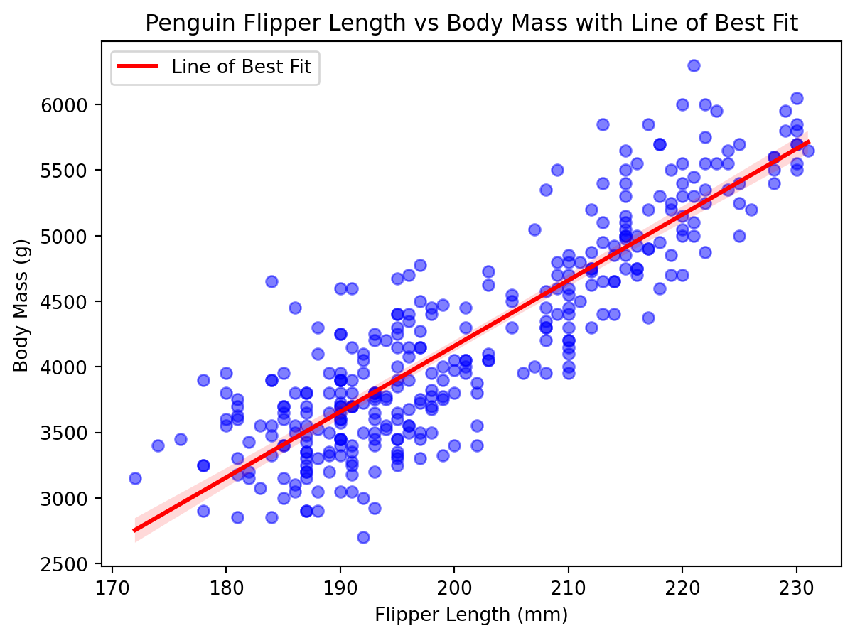
Seaborn provides a convenient way to add a line of best fit to a scatter plot using the regplot function. This function automatically calculates and plots the line of best fit for us.
import seaborn as snsplt.figure(figsize=(7, 5))sns.regplot( x="flipper_length_mm", y="body_mass_g", data=penguins, scatter_kws={"alpha": 0.5, "color": "blue"}, line_kws={"color": "red", "label": "Line of Best Fit"},)plt.xlabel("Flipper Length (mm)")plt.ylabel("Body Mass (g)")plt.title("Penguin Flipper Length vs Body Mass with Line of Best Fit")plt.legend()plt.show()
As in all things python visualizations, seaborn makes it much easier to create complex plots with less code. The regplot function automatically calculates the line of best fit and adds it to the scatter plot, allowing us to visualize the relationship between the two numerical variables easily. Moreover, it also includes confidence intervals for the regression line by default, which can provide additional insights into the uncertainty of the estimates. The light red shaded area around the line represents the confidence interval, indicating the range within which we can expect the true regression line to fall with a certain level of confidence (typically 95%).
When we pass in the scatter_kws and line_kws parameters, we can customize the appearance of the scatter points and the regression line, respectively. In this example, we set the scatter points to be blue with an alpha of 0.5 and the regression line to be red with a label.