9.5 Project

Univariate Visualizations

Note

Download the dataset for this project here: Data Download

Let’s get started by importing the necessary libraries and data.

import pandas as pd
import matplotlib.pyplot as plt
import seaborn as sns

df = pd.read_csv("soccer-player-heights.csv")
df.head()

	player_id	first_name	last_name	name	last_season	current_club_id	player_code	country_of_birth	city_of_birth	country_of_citizenship	...	foot	height_in_cm	contract_expiration_date	agent_name	image_url	url	current_club_domestic_competition_id	current_club_name	market_value_in_eur	highest_market_value_in_eur
0	10	Miroslav	Klose	Miroslav Klose	2015	398	miroslav-klose	Poland	Opole	Germany	...	right	184.0	NaN	ASBW Sport Marketing	https://img.a.transfermarkt.technology/portrai...	https://www.transfermarkt.co.uk/miroslav-klose...	IT1	Società Sportiva Lazio S.p.A.	1000000.0	30000000.0
1	26	Roman	Weidenfeller	Roman Weidenfeller	2017	16	roman-weidenfeller	Germany	Diez	Germany	...	left	190.0	NaN	Neubauer 13 GmbH	https://img.a.transfermarkt.technology/portrai...	https://www.transfermarkt.co.uk/roman-weidenfe...	L1	Borussia Dortmund	750000.0	8000000.0
2	65	Dimitar	Berbatov	Dimitar Berbatov	2015	1091	dimitar-berbatov	Bulgaria	Blagoevgrad	Bulgaria	...	NaN	NaN	NaN	CSKA-AS-23 Ltd.	https://img.a.transfermarkt.technology/portrai...	https://www.transfermarkt.co.uk/dimitar-berbat...	GR1	Panthessalonikios Athlitikos Omilos Konstantin...	1000000.0	34500000.0
3	77	NaN	Lúcio	Lúcio	2012	506	lucio	Brazil	Brasília	Brazil	...	NaN	NaN	NaN	NaN	https://img.a.transfermarkt.technology/portrai...	https://www.transfermarkt.co.uk/lucio/profil/s...	IT1	Juventus Football Club	200000.0	24500000.0
4	80	Tom	Starke	Tom Starke	2017	27	tom-starke	East Germany (GDR)	Freital	Germany	...	right	194.0	NaN	IFM	https://img.a.transfermarkt.technology/portrai...	https://www.transfermarkt.co.uk/tom-starke/pro...	L1	FC Bayern München	100000.0	3000000.0

5 rows × 23 columns

df = df[["player_id", "name", "country_of_citizenship", "date_of_birth", "height_in_cm", "position"]]
df = df.dropna(subset=["height_in_cm", "date_of_birth"])
df.head()

	player_id	name	country_of_citizenship	date_of_birth	height_in_cm	position
0	10	Miroslav Klose	Germany	1978-06-09 00:00:00	184.0	Attack
1	26	Roman Weidenfeller	Germany	1980-08-06 00:00:00	190.0	Goalkeeper
4	80	Tom Starke	Germany	1981-03-18 00:00:00	194.0	Goalkeeper
7	132	Tomas Rosicky	Czech Republic	1980-10-04 00:00:00	179.0	Midfield
8	162	Marc Ziegler	Germany	1976-06-13 00:00:00	193.0	Goalkeeper

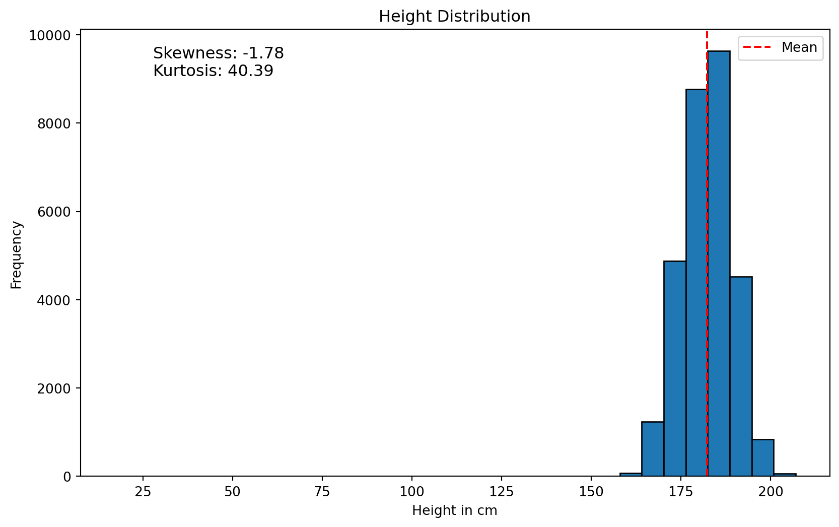
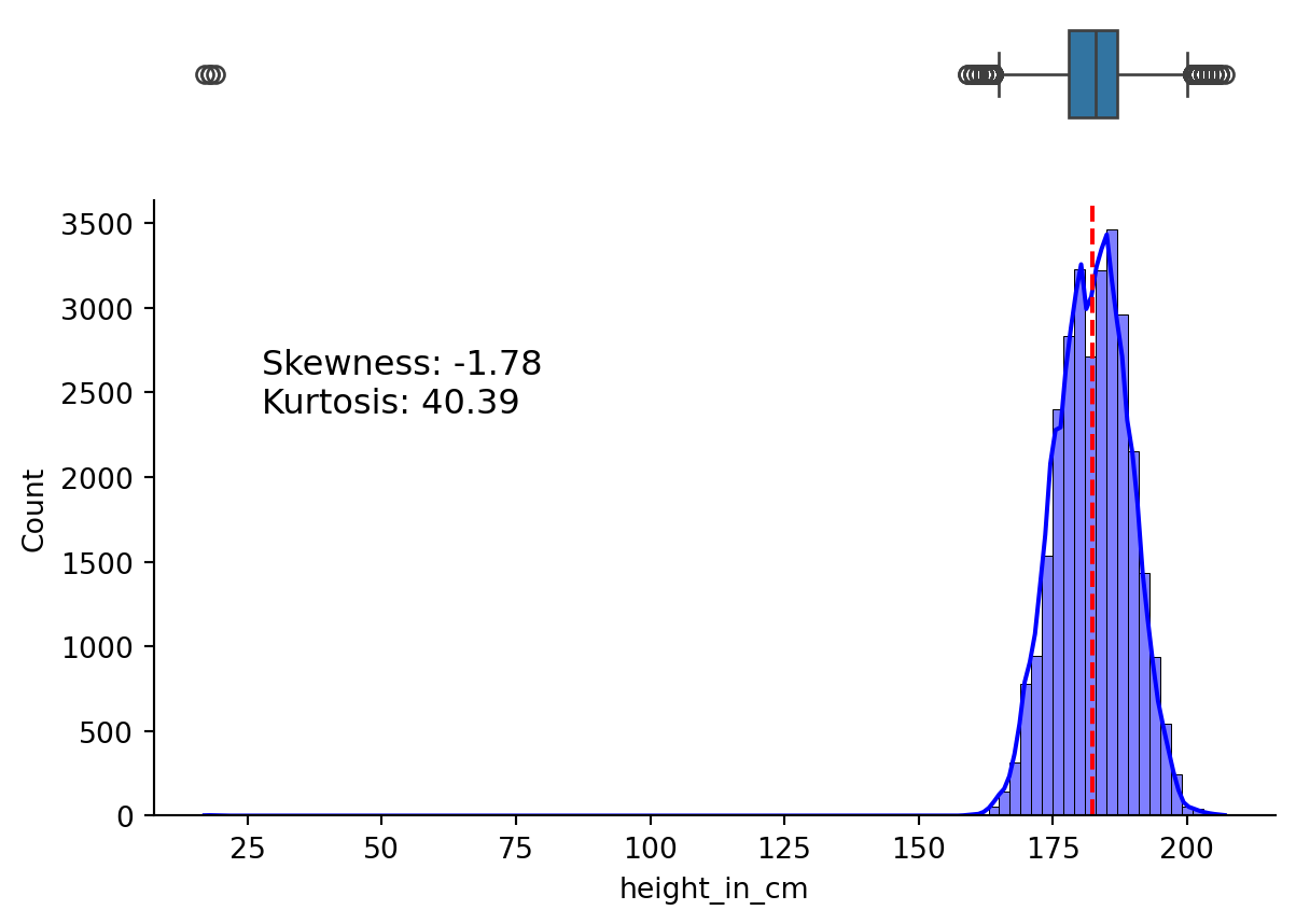
Let’s start by understanding the distribution of heights in the dataset. The first way to look at this is by using a histogram. Let’s start by creating the histogram in matplotlib.

import scipy.stats as stats

skewness = stats.skew(df["height_in_cm"])
kurtosis = stats.kurtosis(df["height_in_cm"])

plt.figure(figsize=(10, 6))
bins = int(df["height_in_cm"].count() ** (1 / 3))
plt.hist(df["height_in_cm"], bins=bins, edgecolor="black")
plt.xlabel("Height in cm")
plt.ylabel("Frequency")
plt.title("Height Distribution")
plt.axvline(df["height_in_cm"].mean(), color="r", linestyle="--", label="Mean")
text = f"Skewness: {skewness:.2f}\nKurtosis: {kurtosis:.2f}"
plt.text(0.2, 0.8, text, fontsize=12, transform=plt.gcf().transFigure)
plt.legend()

plt.show()

Now let’s do this same plot using seaborn.

hp = sns.histplot(data=df, x="height_in_cm", kde=True, color="blue", binwidth=2)
plt.axvline(df["height_in_cm"].mean(), color="r", linestyle="--")
text = f"Skewness: {skewness:.2f}\nKurtosis: {kurtosis:.2f}"
hp.text(0.2, 0.8, text, fontsize=12, transform=plt.gcf().transFigure)
plt.show()

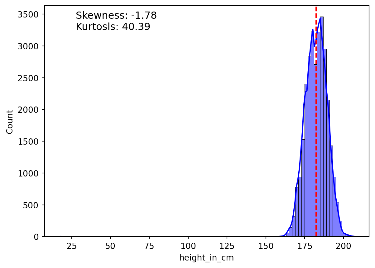
Seaborn makes it much easier by abstracting away much of the calculations. For instance, it creates the Kernel Density Estimation (KDE) plot by default. The KDE plot provides a smoothed estimation of the distribution of the data.

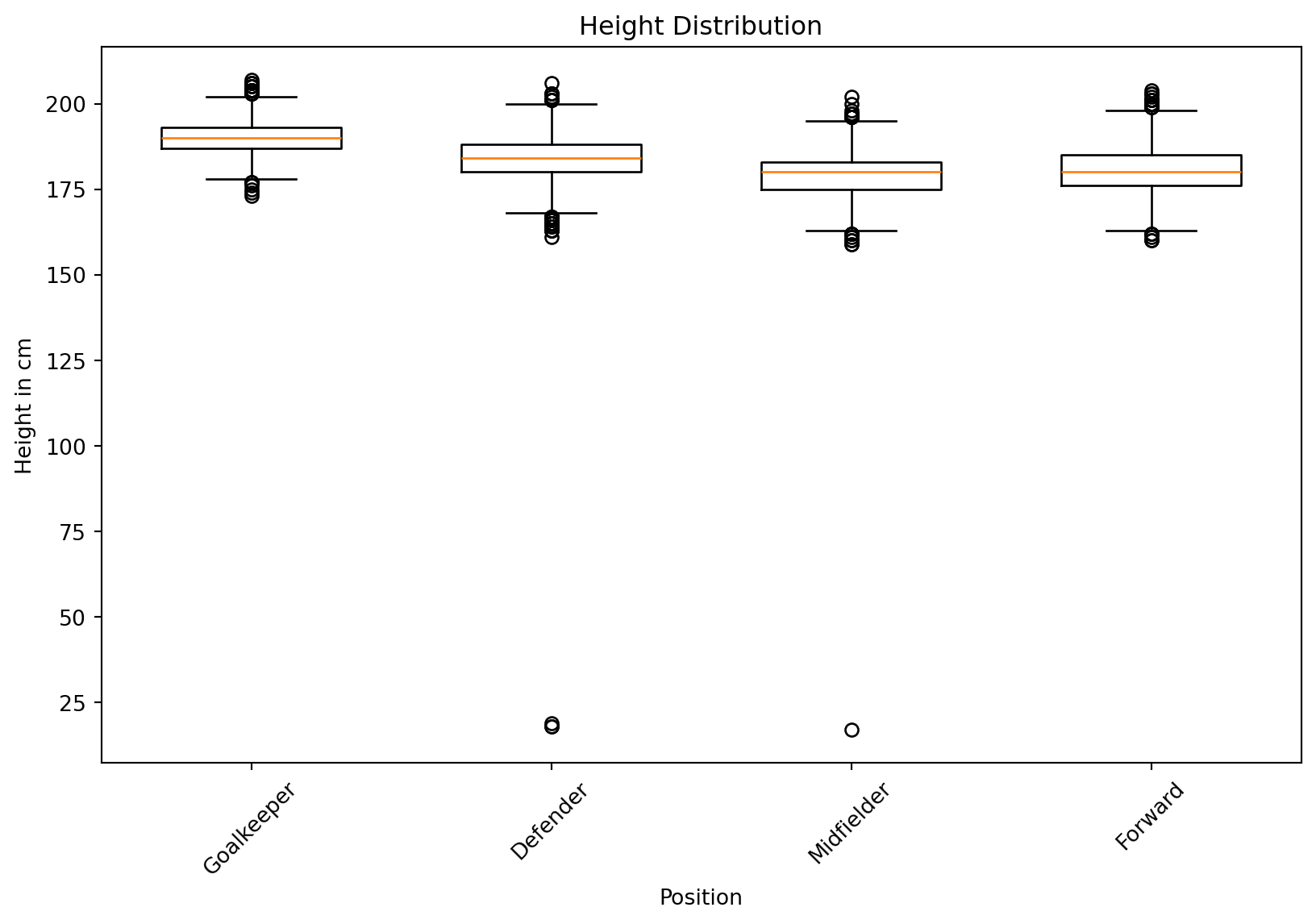
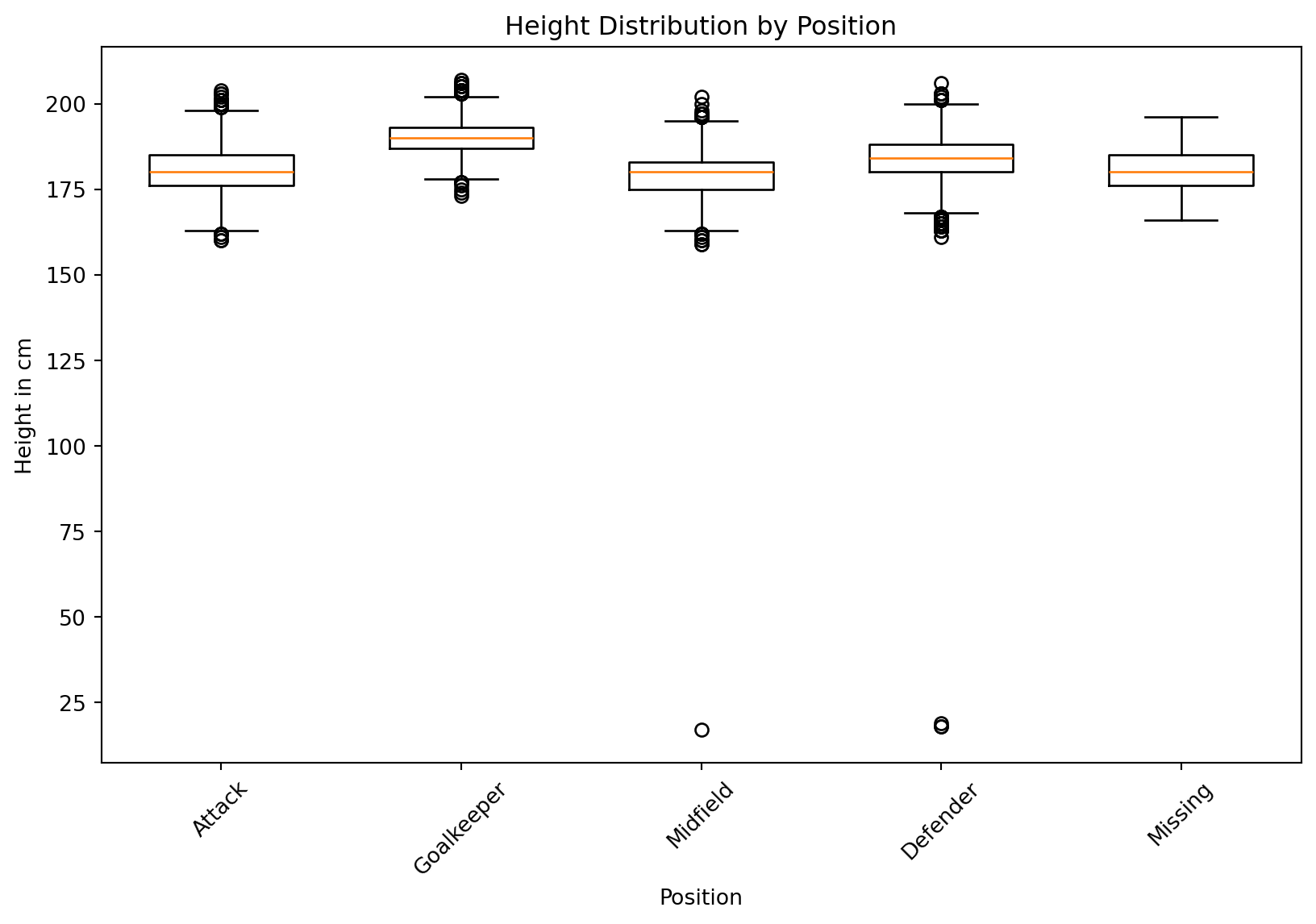
Now let’s create a box plot, but let’s first do it with matplotlib.

plt.figure(figsize=(10, 6))
plt.boxplot(df.loc[df["position"] == "Goalkeeper", "height_in_cm"], 
            positions=[1], widths=0.6)
plt.boxplot(df.loc[df["position"] == "Defender", "height_in_cm"], 
            positions=[2], widths=0.6)
plt.boxplot(df.loc[df["position"] == "Midfield", "height_in_cm"], 
            positions=[3], widths=0.6)
plt.boxplot(df.loc[df["position"] == "Attack", "height_in_cm"], 
            positions=[4], widths=0.6)
plt.xticks(
    [1, 2, 3, 4],
    ["Goalkeeper", "Defender", "Midfielder", "Forward"],
    rotation=45,
)
plt.ylabel("Height in cm")
plt.title("Height Distribution")
plt.xlabel("Position")
plt.show()

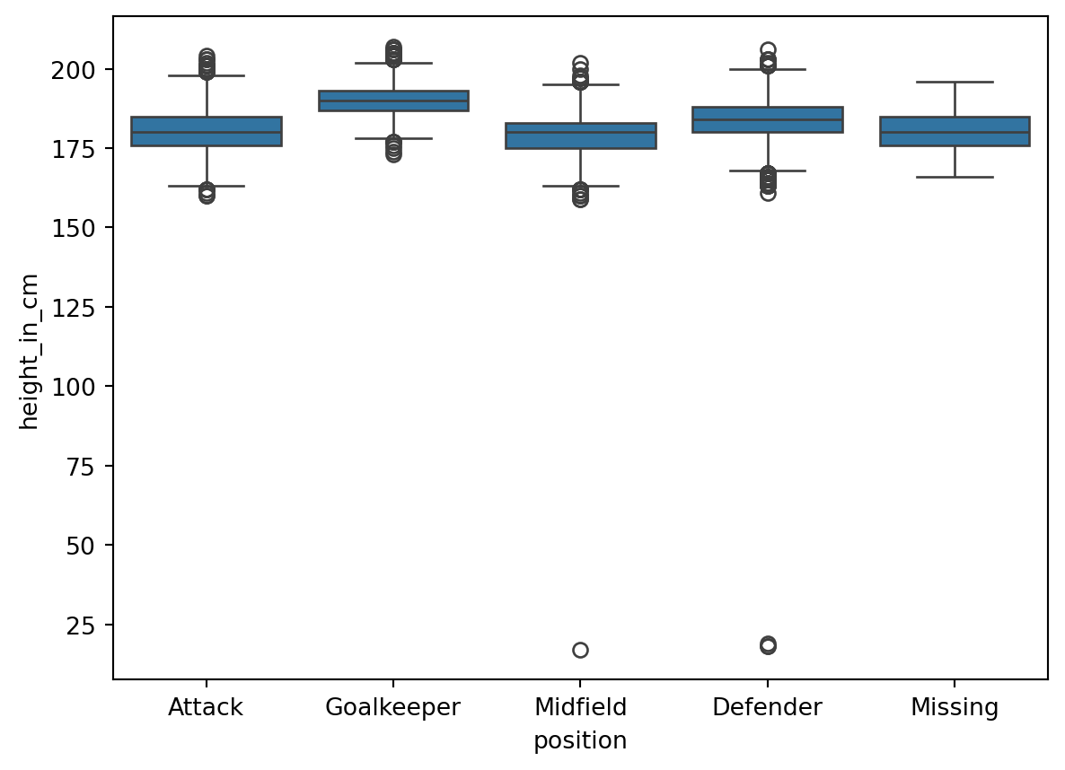
Now let’s remember that the box plot represents the interquartile range (IQR), or the middle 50% of the data. The bottom of the box is the 25th percentile, the line in the middle is the median, and the top of the box is the 75th percentile. The whiskers represent the range of the data, and the points are outliers. Whiskers extend to the most extreme data points within 1.5 times the IQR from the box.

sns.boxplot(y=df["height_in_cm"], x=df["position"])
plt.show()

To do this same thing in matplotlib, we would have to do more work.

positions = df["position"].unique()
plt.figure(figsize=(10, 6))
for i, pos in enumerate(positions):
    plt.boxplot(
        df.loc[df["position"] == pos, "height_in_cm"],
        positions=[i],
        widths=0.6,
    )
plt.xticks(range(len(positions)), positions, rotation=45)
plt.xlabel("Position")
plt.ylabel("Height in cm")
plt.title("Height Distribution by Position")
plt.show()

Multiple Plots

We can also create a combination of a box plot and a histogram by using the subplot function in matplotlib. We can use matplotlib’s subplot method, which permits us to create multiple plots in a single figure. It returns a figure along with a tuple including each plot. Below, I destructured the figure as f, and the tuple as plt1 and plt2.

Then, when we create our plots with seaborn, we assign the ax argument to the plot we want it to be connected to.

f, (plt1, plt2) = plt.subplots(2, gridspec_kw={"height_ratios": (0.15, 0.85)})

sns.boxplot(df["height_in_cm"], ax=plt1, orient="h")
sns.histplot(data=df, x="height_in_cm", ax=plt2, binwidth=2, kde=True, color="blue")

plt1.set(yticks=[])
plt1.set(xticks=[])
plt1.set_xlabel("")
plt.axvline(df["height_in_cm"].mean(), color="r", linestyle="--")
sns.despine(
    ax=plt2,
)
text = f"Skewness: {skewness:.2f}\nKurtosis: {kurtosis:.2f}"
plt2.text(0.2, 0.5, text, fontsize=12, transform=plt.gcf().transFigure)
sns.despine(ax=plt1, left=True, bottom=True)
plt.show()