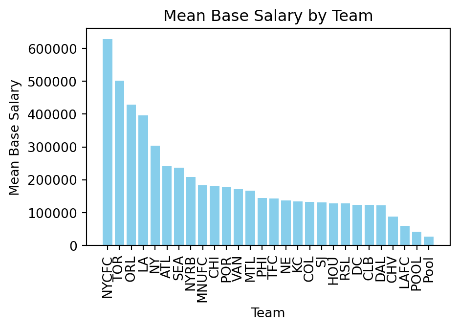
The simplest way to demonstrate differences across categories is to use a basic bar chart. Bar charts display the mean (or sum) of a numeric variable for each category of a categorical variable.
Let’s start by loading in a dataset. This time let’s look at data of Major League Soccer (MLS) players salaries. We will use this dataset to compare player salaries across different positions and teams.
import pandas as pdurl ="https://raw.githubusercontent.com/nkmwicz/data-for-students/refs/heads/main/mls-salaries.csv"df = pd.read_csv(url)df.head()
club
last_name
first_name
position
base_salary
guaranteed_compensation
year
0
CHI
Armas
Chris
M
225000.0
225000.0
2007
1
CHI
Banner
Michael
M
12900.0
12900.0
2007
2
CHI
Barrett
Chad
F
41212.5
48712.5
2007
3
CHI
Blanco
Cuauhtemoc
F
2492316.0
2666778.0
2007
4
CHI
Brown
C.J.
D
106391.0
106391.0
2007
Now we can see that we have the team, name, position, base salary, guaranteed compensation, and year categories. This provides us with a number of ways that we can compare salaries across different groups.
To begin with, let’s create a simple bar chart that compares the mean base salary across different teams. To do this analysis, we have to group the data by team and then aggregate the data with agg() to calculate the mean base salary and guaranteed compensation for each team.
By using a named tuple in the agg() function, we can create new column names for our aggregated data.
Now that the data is in the proper formate, we can begin to create our bar chart.
We can use both seaborn and matplotlib to create this visualization. We will start with matplotlib, using the bar function.
The bar function takes two primary arguments:
import matplotlib.pyplot as pltteams_df = teams_df.sort_values("base", ascending=False)plt.figure(figsize=(5, 3))teams = teams_df.indexsalaries = teams_df["base"]plt.bar(teams, salaries, color="skyblue")plt.title("Mean Base Salary by Team")plt.xlabel("Team")plt.ylabel("Mean Base Salary")plt.xticks(rotation=90)plt.show()
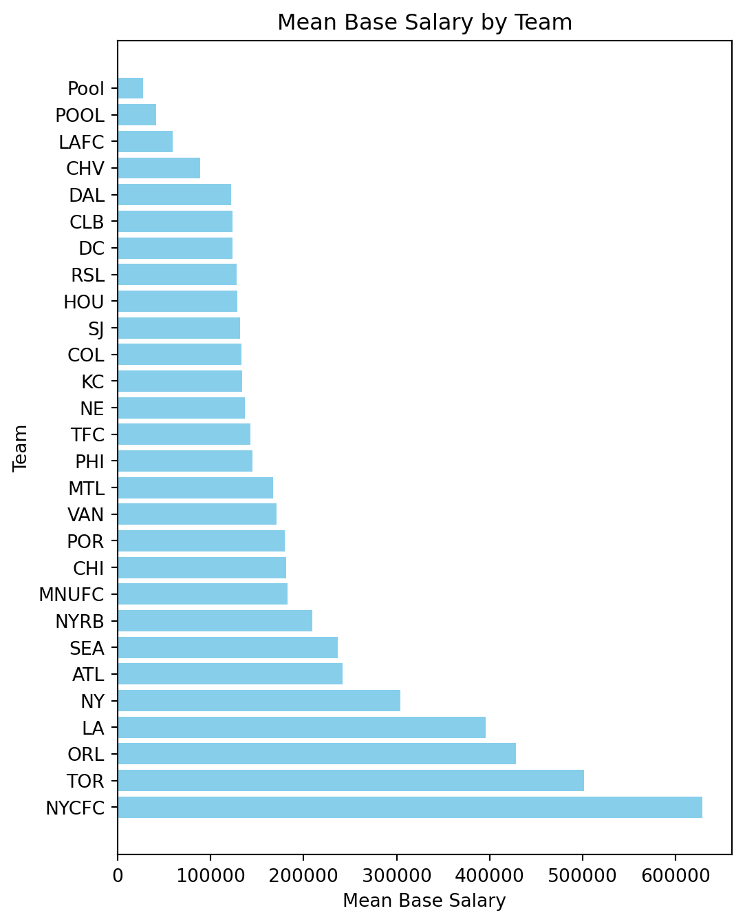
There are ways to improve the visualization. Since we have so many columns. There are 28 teams in the dataset, we may want to increase the figure size and make it vertically oriented to make it easier to read. Luckily, matplotlib has a barh function that creates horizontal bar charts. Let’s use that instead.
plt.figure(figsize=(6, 8))plt.barh(teams, salaries, color="skyblue")plt.title("Mean Base Salary by Team")plt.xlabel("Mean Base Salary")plt.ylabel("Team")plt.show()
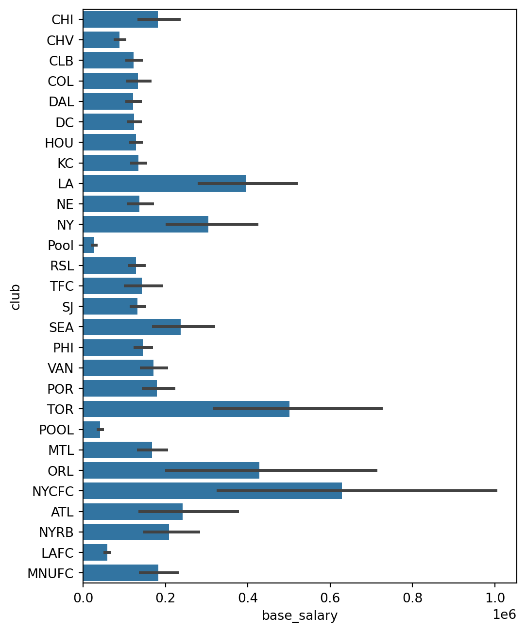
It’s always important to understand how to work in matplotlib because we are able to customize it so much. Nevertheless, but seaborn makes it even easier to create bar charts. We can use the barplot function from seaborn to create the same chart with less code.
Bar Plots in Seaborn
In seaborn, we can use the barplot function to create bar charts. The barplot function takes the data frame, the x-axis variable, and the y-axis variable as arguments. With seaborn,
import seaborn as snsplt.figure(figsize=(6, 8))sns.barplot(x="base_salary", y="club", data=df)